LightTune: Lightweight Forward-Only Online Fine-Tuning with Applications to Link Adaptation
Pith reviewed 2026-05-22 11:02 UTC · model grok-4.3
The pith
LightTune enables backpropagation-free online fine-tuning of ML models on devices by updating only when live performance drops below a set threshold.
A machine-rendered reading of the paper's core claim, the machinery that carries it, and where it could break.
Core claim
LightTune is a lightweight, backpropagation-free online fine-tuning framework with provable convergence guarantees that opportunistically refines ML models using live test-time data only when performance falls below a predefined threshold, enabling dynamic adaptation to previously unseen channel conditions in 6G mobile systems with up to 48.8 percent reduction in average BLER prediction error and up to 15.5 percent average throughput improvement over table-based outer loop link adaptation.
What carries the argument
The threshold-triggered forward-only update rule that refines model parameters without gradients while preserving convergence.
If this is right
- ML-based BLER predictors can maintain accuracy across changing wireless environments without full retraining.
- Link adaptation can shift from static tables to adaptive models while keeping compute costs low on mobile hardware.
- Similar forward-only updates could stabilize other real-time prediction tasks that face distributional shift.
- The convergence guarantees reduce the risk of instability when deploying the method in live networks.
Where Pith is reading between the lines
- The same lightweight adaptation pattern could be tested on other edge tasks such as sensor fusion or speech recognition where conditions drift over time.
- If the threshold logic generalizes, it may reduce reliance on collecting massive offline datasets for every possible environment.
- Extending the approach to multi-model systems could allow coordinated adaptation across different layers of a wireless stack.
Load-bearing premise
Live test-time data remains representative of new conditions and the chosen performance threshold reliably triggers updates that converge for the prediction task.
What would settle it
A test in which the fine-tuned model shows no reduction in BLER prediction error or throughput gain when deployed on channel conditions that differ markedly from those used to trigger the updates.
Figures



read the original abstract
Deploying machine learning (ML) algorithms on mobile phones is bottlenecked by performance degradation under dynamic, real-world conditions that differ from the offline training conditions. While continual learning and adaptation are essential to mitigate this distributional shift, conventional online learning methods are often computationally prohibitive for resource-constrained devices. In this paper, we propose LightTune, a lightweight, backpropagation-free online fine-tuning framework with provable convergence guarantees. LightTune opportunistically refines ML models using live test-time data only when performance falls below a predefined threshold, ensuring minimal computational overhead and highly efficient responsiveness. As a practical demonstration, we integrate LightTune into a block error rate (BLER) prediction algorithm for 6G mobile systems. This integration enables the ML BLER prediction model to dynamically adapt to previously unseen channel conditions in real-time. Our extensive results show a substantial reduction in the average BLER prediction error of up to 48.8% with online fine-tuning. Furthermore, we leverage this BLER prediction algorithm for link adaptation and demonstrate average throughput improvements of up to 15.5% compared to a conventional table-based outer loop link adaptation (OLLA) algorithm.
Editorial analysis
A structured set of objections, weighed in public.
Referee Report
Summary. The manuscript proposes LightTune, a lightweight backpropagation-free online fine-tuning framework that opportunistically updates ML models using only live test-time data when performance drops below a threshold, with claimed provable convergence guarantees. It applies this to a BLER prediction model for 6G link adaptation, reporting up to 48.8% reduction in average BLER prediction error and 15.5% average throughput gain over conventional table-based OLLA.
Significance. If the lightweight adaptation mechanism and convergence guarantees are rigorously validated, particularly under dynamic wireless conditions, the work could meaningfully advance practical deployment of ML models on resource-constrained mobile devices by addressing distributional shift with minimal overhead.
major comments (2)
- [§3.2] §3.2 (Convergence Analysis): The proof sketch for threshold-triggered forward-only updates relies on assumptions typical of stationary or slowly varying distributions; this is load-bearing for the central claim of provable convergence in previously unseen, dynamic 6G channel conditions. The manuscript should explicitly address or test robustness to abrupt non-stationary shifts.
- [§5.3] §5.3 (Experimental Results): The reported 48.8% BLER error reduction and 15.5% throughput improvement are presented without sufficient detail on the number of Monte Carlo trials, exact channel models for unseen conditions, statistical variance, or comparisons to other lightweight online methods; this undermines verification of the empirical claims.
minor comments (2)
- [Abstract] Abstract: Consider adding one sentence on the specific form of the forward-only update rule to improve accessibility.
- [§2] Notation: Ensure consistent definition of the performance threshold parameter across sections; it is introduced informally in the abstract.
Simulated Author's Rebuttal
We thank the referee for their thorough review and constructive suggestions. We address each of the major comments in detail below, indicating where we plan to revise the manuscript to incorporate the feedback.
read point-by-point responses
-
Referee: [§3.2] §3.2 (Convergence Analysis): The proof sketch for threshold-triggered forward-only updates relies on assumptions typical of stationary or slowly varying distributions; this is load-bearing for the central claim of provable convergence in previously unseen, dynamic 6G channel conditions. The manuscript should explicitly address or test robustness to abrupt non-stationary shifts.
Authors: We appreciate this observation regarding the convergence analysis. The proof in Section 3.2 is developed under standard assumptions for analyzing the convergence of the forward-only update rule, which include stationary distributions to establish the guarantees. However, the design of LightTune, with its performance-threshold trigger, is specifically intended to respond to distributional shifts, including those in dynamic wireless environments. To address the referee's concern, we will revise the manuscript to include an explicit discussion of these assumptions and their applicability to non-stationary conditions. Additionally, we will add new simulation results demonstrating the method's performance under abrupt channel shifts in the experimental section. revision: yes
-
Referee: [§5.3] §5.3 (Experimental Results): The reported 48.8% BLER error reduction and 15.5% throughput improvement are presented without sufficient detail on the number of Monte Carlo trials, exact channel models for unseen conditions, statistical variance, or comparisons to other lightweight online methods; this undermines verification of the empirical claims.
Authors: We agree that providing more details on the experimental setup would improve the clarity and verifiability of our results. In the revised manuscript, we will expand Section 5.3 to specify the number of Monte Carlo trials performed, provide exact parameters for the channel models used to simulate unseen conditions, report statistical measures such as variance or confidence intervals for the reported improvements, and include comparisons against additional lightweight online adaptation methods from the literature. revision: yes
Circularity Check
No circularity: empirical claims rest on experimental outcomes, not self-referential derivations
full rationale
The paper introduces LightTune as a backpropagation-free online fine-tuning method triggered by a performance threshold, claiming provable convergence guarantees and reporting empirical gains (up to 48.8% BLER error reduction and 15.5% throughput improvement). No equations, fitted parameters renamed as predictions, or load-bearing self-citations appear in the abstract or description. The central results are presented as measured outcomes from live test-time adaptation experiments rather than theoretical reductions that equate outputs to inputs by construction. The derivation chain is therefore self-contained as an empirical framework without the circular patterns enumerated in the guidelines.
Axiom & Free-Parameter Ledger
Lean theorems connected to this paper
-
IndisputableMonolith/Cost/FunctionalEquation.leanwashburn_uniqueness_aczel unclear?
unclearRelation between the paper passage and the cited Recognition theorem.
We propose LightTune, a lightweight, backpropagation-free online fine-tuning framework with provable convergence guarantees. LightTune opportunistically refines ML models using live test-time data only when performance falls below a predefined threshold
-
IndisputableMonolith/Foundation/ArithmeticFromLogic.leanabsolute_floor_iff_bare_distinguishability unclear?
unclearRelation between the paper passage and the cited Recognition theorem.
the average frequency of prediction errors reaching or exceeding any fixed threshold δ converges to 0 as the number of fine-tuning steps increases
What do these tags mean?
- matches
- The paper's claim is directly supported by a theorem in the formal canon.
- supports
- The theorem supports part of the paper's argument, but the paper may add assumptions or extra steps.
- extends
- The paper goes beyond the formal theorem; the theorem is a base layer rather than the whole result.
- uses
- The paper appears to rely on the theorem as machinery.
- contradicts
- The paper's claim conflicts with a theorem or certificate in the canon.
- unclear
- Pith found a possible connection, but the passage is too broad, indirect, or ambiguous to say the theorem truly supports the claim.
Reference graph
Works this paper leans on
-
[1]
LightTune: Lightweight Online Fi ne-Tuning for 6G,
R. E. Ali and F. Penna, “LightTune: Lightweight Online Fi ne-Tuning for 6G,” in IEEE International Conference on Communications (ICC) , 2026
work page 2026
-
[2]
Study on Ar tificial In- telligence (AI)/Machine Learning (ML) for NR Air Interface ,
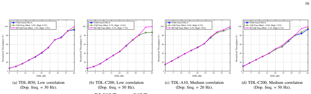
3rd Generation Partnership Project (3GPP), “Study on Ar tificial In- telligence (AI)/Machine Learning (ML) for NR Air Interface ,” 3GPP , Technical Report 38.843, Release 18, 2023. Medium SNR Gain High SNR Gain Channel CQI-Tune RI-CQI-Tune CQI-Tune RI-CQI-Tune TDL-B50, 30 Hz (Low Corr.) 2% 1% 0 . 2% 1 . 8% TDL-C200, 50 Hz (Low Corr.) 0. 7% 0 . 1% − 0. 2% 7...
work page 2023
-
[3]
Statistical AI/ML model monitoring for 5G/6G: Interference prediction case study,
P . Kaswan et al. , “Statistical AI/ML model monitoring for 5G/6G: Interference prediction case study,” in IEEE International Conference on Communications W orkshops (ICC W orkshops), 2024
work page 2024
-
[4]
Learning to estimate: A real-time online learning frame- work for MIMO-OFDM channel estimation,
J. Xu et al. , “Learning to estimate: A real-time online learning frame- work for MIMO-OFDM channel estimation,” IEEE Transactions on Wireless Communications, 2024
work page 2024
-
[5]
Learning at the speed of wireless: Online real-time learning for AI-enabled MIMO in NextG,
——, “Learning at the speed of wireless: Online real-time learning for AI-enabled MIMO in NextG,” IEEE Communications Magazine , 2024
work page 2024
-
[6]
AI/ML Use Cases and Framework for 6GR,
Samsung, “AI/ML Use Cases and Framework for 6GR,” 3GPP TS G RAN1 Meeting #122, Bengaluru, India, R1-2505588, Aug. 2025
work page 2025
-
[7]
Reinforcement l earning for efficient and tuning-free link adaptation,
V . Saxena, H. Tullberg, and J. Jald´ en, “Reinforcement l earning for efficient and tuning-free link adaptation,” IEEE Transactions on Wireless Communications, vol. 21, no. 2, 2021
work page 2021
-
[8]
DRAGON: A DRL-based MIMO Layer and MCS Adapter in Open RAN 5G Networks,
Q. An et al. , “DRAGON: A DRL-based MIMO Layer and MCS Adapter in Open RAN 5G Networks,” in Proceedings of the 30th Annual International Conference on Mobile Computing and Networki ng, 2024
work page 2024
-
[9]
The forward-forward algorithm: Some preliminary investigations
G. Hinton, “The Forward-Forward Algorithm: Some Prelim inary Inves- tigations,” arXiv preprint arXiv:2212.13345 , 2022
-
[10]
Self-improving reactive agents based on re inforcement learn- ing, planning and teaching,
L.-J. Lin, “Self-improving reactive agents based on re inforcement learn- ing, planning and teaching,” Machine learning , vol. 8, no. 3, 1992
work page 1992
-
[11]
Prioritized Experience Replay,
T. Schaul et al. , “Prioritized Experience Replay,” ICLR, 2016
work page 2016
-
[12]
Experience Replay for Continual Learning,
D. Rolnick et al., “Experience Replay for Continual Learning,” Advances in neural information processing systems , vol. 32, 2019
work page 2019
-
[13]
Outer loop link adaptation enhancements for ultra reliable low latency communications in 5G,
E. Peralta et al. , “Outer loop link adaptation enhancements for ultra reliable low latency communications in 5G,” in IEEE 95th V ehicular Technology Conference:(VTC-Spring), 2022
work page 2022
-
[14]
Machine learning based link adaptation method for MIMO system,
Z. Dong et al. , “Machine learning based link adaptation method for MIMO system,” in IEEE 29th Annual International Symposium on Personal, Indoor and Mobile Radio Communications (PIMRC) , 2018
work page 2018
-
[15]
Machine-learning-aided link-per formance pre- diction for coded MIMO systems,
T. V an Le and K. Lee, “Machine-learning-aided link-per formance pre- diction for coded MIMO systems,” IEEE Transactions on V ehicular Technology, vol. 71, no. 3, 2021
work page 2021
-
[16]
Online Adaptation and ML-Non-ML C ombin- ing for Improved Wireless Link Adaptation,
R. E. Ali and H. Kwon, “Online Adaptation and ML-Non-ML C ombin- ing for Improved Wireless Link Adaptation,” US Patent, 2026
work page 2026
-
[17]
Adaptive CQI and RI Estimation f or 5G NR: A Shallow Reinforcement Learning Approach,
A. Baknina and H. Kwon, “Adaptive CQI and RI Estimation f or 5G NR: A Shallow Reinforcement Learning Approach,” in IEEE Global Communications Conference (GLOBECOM) , 2020
work page 2020
-
[18]
DELUXE: A DL-based link adaptation for URLLC/eMBB multiplexing in 5G NR,
Y . Huang, Y . T. Hou, and W. Lou, “DELUXE: A DL-based link adaptation for URLLC/eMBB multiplexing in 5G NR,” IEEE Journal on Selected Areas in Communications , vol. 40, no. 1, 2021
work page 2021
-
[19]
Enhancing olla via exponential decay for efficient link ada ptation in emerging 6g traffic,
A. Mazumdar, S. Paris, A. Amiri, K. I. Pedersen, and R. Ad eogun, “Enhancing olla via exponential decay for efficient link ada ptation in emerging 6g traffic,” IEEE Access , vol. 14, pp. 5764–5776, 2026
work page 2026
-
[20]
Salad: Self-adaptive link adaptation,
R. Wiesmayr, L. Maggi, S. Cammerer, J. Hoydis, F. A. Aoud ia, and A. Keller, “Salad: Self-adaptive link adaptation,” arXiv preprint arXiv:2510.05784, 2025
-
[21]
Sinr estimation under limited feedback via online convex optimi zation,
L. Maggi, B. Bonev, R. Wiesmayr, S. Cammerer, and A. Kell er, “Sinr estimation under limited feedback via online convex optimi zation,” arXiv preprint arXiv:2603.02061, 2026
-
[22]
On Advancements of the Forward-Forward Algorithm,
M. O. Torres, M. Lange, and A. P . Raulf, “On Advancements of the Forward-Forward Algorithm,” arXiv preprint arXiv:2504.21662 , 2025
-
[23]
Facenet: A unified embed- ding for face recognition and clustering,
F. Schroff, D. Kalenichenko, and J. Philbin, “Facenet: A unified embed- ding for face recognition and clustering,” in Proceedings of the IEEE conference on computer vision and pattern recognition , 2015
work page 2015
-
[24]
Adam: A method for stochastic opt imization,
D. P . Kingma and J. Ba, “Adam: A method for stochastic opt imization,” in International Conference on Learning Representations (IC LR), 2015
work page 2015
-
[25]
H. Karimi, J. Nutini, and M. Schmidt, “Linear convergen ce of gradient and proximal-gradient methods under the polyak-łojasiewi cz condition,” 14 in Joint European conference on machine learning and knowledg e discovery in databases . Springer, 2016, pp. 795–811
work page 2016
-
[26]
Nesterov, Introductory lectures on convex optimization: A basic course
Y . Nesterov, Introductory lectures on convex optimization: A basic course. Springer Science & Business Media, 2013, vol. 87
work page 2013
-
[27]
Information and information stability of random vari- ables and processes,
M. S. Pinsker, “Information and information stability of random vari- ables and processes,” Holden-Day, 1964
work page 1964
-
[28]
Physical layer procedures for data (release 16) ,
3GPP , “Physical layer procedures for data (release 16) ,” Technical Specification (TS) 38.214, 2021
work page 2021
-
[29]
TinyFoA: Memory efficient for ward- only algorithm for on-device learning,
B. Huang and A. Aminifar, “TinyFoA: Memory efficient for ward- only algorithm for on-device learning,” in Proceedings of the AAAI Conference on Artificial Intelligence , 2025
work page 2025
-
[30]
µ -FF: on-device forward-forward training algorithm for microcontrollers,
F. De Vita et al. , “ µ -FF: on-device forward-forward training algorithm for microcontrollers,” in IEEE Conference on Smart Computing , 2023
work page 2023
-
[31]
Study on channel model for frequencies from 0.5 t o 100 GHz,
3GPP , “Study on channel model for frequencies from 0.5 t o 100 GHz,” Tech. Rep. TR 38.901 V14.0.0, July 2017
work page 2017
-
[32]
User equipment (UE) radio transmission and rece ption,
3GPP, “User equipment (UE) radio transmission and rece ption,” Tech. Rep. TS 36.101, 2024
work page 2024
-
[33]
Gradient-based learning applied to document recogni- tion,
Y . LeCun et al. , “Gradient-based learning applied to document recogni- tion,” Proc. IEEE , vol. 86, no. 11, 1998
work page 1998
-
[34]
Implementation of Forward-Forward (FF) training algo- rithm,
M. Pezeshki, “Implementation of Forward-Forward (FF) training algo- rithm,” https://github.com/mpezeshki/pytorch forward forward, 2023
work page 2023
-
[35]
R. A. Horn and C. R. Johnson, Matrix analysis . Cambridge university press, 2012. APPENDIX A THEORETICAL INSIGHTS AND EXPERIMENTAL VALIDATION OF THE PROPOSED LOSS FUNCTION We derive our alternative quadratic loss from the second- order Taylor expansion of the function f (x) = ln(1 + ex), centered at x = 0 that is given as f (x) = ln 2 + 1 2 x + 1 8 x2 + R...
work page 2012
-
[36]
and subsequently extended in [16]. We briefly describe the scheme of [16], which employs an MLP to predict the spectral efficiency (SE) for all possible RI and CQI candidat e pairs, and subsequently selects the pair that maximizes the estimated SE. To mitigate training-test mismatch, the reco rded ACKs/NACKs are leveraged to compute an empirical SE esti- ma...
-
[37]
(47) Thus it suffices to bound the Hessian of a single neuron; the full Hessian norm will be at most that bound divided by Ml. d) Bounding the per-neuron Hessian.: Fix a neuron j and time t, and drop the indices l, j, t for brevity. When p+ > 0 (neuron active), we have ∇L + = [ 4p3 +− 4(T + 2)p+ ]˜h+. (48) Differentiating again with respect to θ (using ∂p ...
-
[38]
Points where the gradient may not be differentiable. For each neuron k in layer l, its pre-activation along the segment is pk(s) = θl,k (s)⊤ ˜hl− 1, (56) where θl,k (s) is the part of θ (s) corresponding to neuron k, and ˜hl− 1 is fixed (it comes from the sample at time t and does not depend on s). This is an affine function of s, i.e., pk(s) = aks + bk for...
-
[39]
For a fixed k, the equation pk(s) = 0 is linear in s
Zeros of affine functions are isolated. For a fixed k, the equation pk(s) = 0 is linear in s. Hence it has either: 1) no solution (if ak = 0 and bk̸= 0), 2) exactly one solution s∗ k (if ak ̸= 0 ) or 3) the whole interval (if ak = 0 and bk = 0, which would mean the pre-activation is identically zero; this degenerate case occurs on a set of measure zero and ...
-
[40]
Since there are finitely many neurons, the set S0 ={s∈ [0, 1] :∃k such that pk(s) = 0} (57) is finite
The exceptional set is finite. Since there are finitely many neurons, the set S0 ={s∈ [0, 1] :∃k such that pk(s) = 0} (57) is finite. Order its elements as 0≤ s1 <··· < s m ≤
-
[41]
Remove these points to obtain a partition of [0, 1] into subintervals [0, s 1], [s1, s 2], . . . , [sm, 1]. On each such subinterval, no pre-activation changes sign, so the activation pattern (which neurons are active) remain s fixed. Consequently, on each subinterval, the gradient ∇L (t) l (θ (s)) is a polynomial in s (because the per-neuron contributions...
-
[42]
Derivative on a smooth subinterval. On any subinterval where∇L (t) l (θ (s)) is C1, we can differentiate: d ds∇L (t) l (θl(s)) =∇ 2L(t) l (θl(s)) (θ ′ l− θl), (58) where the Hessian exists everywhere on the interval be- cause the activation pattern is constant. From the bound on the Hessian, we have ∥∇ 2L(t) l (θl(s))∥2≤ ρl, so d ds∇L (t) l (θl(s)...
-
[43]
Apply the funda- mental theorem of calculus on each subinterval
Integration over each subinterval. Apply the funda- mental theorem of calculus on each subinterval. Because ∇L (t) l (θ (s)) is continuously differentiable on the open interval and continuous up to the endpoints, we have ∇L (t) l (θl(si+1))−∇L (t) l (θl(si)) = ∫ si+1 si ∇ 2L(t) l (θl(s)) (θ ′ l− θl) ds. Summing these equalities from i = 0 to m (with s0 = ...
-
[44]
Norm estimate. Taking norms and using the triangle inequality, ∥∇L (t) l (θ ′ l)−∇L (t) l (θl)∥2 ≤ m∑ i=0 ∫ si+1 si ∥∇ 2L(t) l (θl(s))∥2∥θ ′ l− θl∥2 ds ≤ ρl∥θ ′ l− θl∥2 m∑ i=0 (si+1− si) = ρl∥θ ′ l− θl∥2. Thus,L(t) l is ρl-smooth. D. Convergence Theorem We now provide the proof of Theorem 1. Proof. We proceed in steps as follows
-
[45]
Local decrease. For any t, if I (t) δ = 1 , the algorithm performs a gradient update: θ (t+1) L = θ (t) L − α f∇L (t) L (θ (t) L ). (60) BecauseL(t) L is ρL-smooth (Lemma 4), we can apply the descent lemma (Lemma 5) with θ = θ (t) L and θ ′ = θ (t+1) L : L(t) L (θ (t+1) L )≤L (t) L (θ (t) L ) +∇L (t) L (θ (t) L )⊤ (θ (t+1) L − θ (t) L ) + ρL 2∥θ (t+1) L −...
-
[46]
(63) Since α f < 1/ρ L, we have ρ Lα f 2 < 1 2 , hence 1− ρ Lα f 2 > 1 2
(61) 19 Substituting the update θ (t+1) L − θ (t) L =− α f∇L (t) L (θ (t) L ) gives L(t) L (θ (t+1) L )≤L (t) L (θ (t) L )− α f∥∇L (t) L (θ (t) L )∥2 2 + ρLα 2 f 2 ∥∇L (t) L (θ (t) L )∥2 2 (62) =L(t) L (θ (t) L )− α f ( 1− ρLα f 2 ) ∥∇L (t) L (θ (t) L )∥2 2. (63) Since α f < 1/ρ L, we have ρ Lα f 2 < 1 2 , hence 1− ρ Lα f 2 > 1 2 . Therefore, L(t) L (θ (t...
-
[47]
(64) If I (t) δ = 0, no update occurs, so L(t) L (θ (t+1) L ) =L(t) L (θ (t) L ). Combining both cases yields L(t) L (θ (t+1) L )≤L (t) L (θ (t) L )− α f 2∥∇L (t) L (θ (t) L )∥2 2I (t) δ . (65)
-
[48]
Conditional expectation under D2. Conditioning on Ft (which fixes θ (t) L , x(t), y(t) + ) and using the gradient lower bound (Assumption 4), Ey(t) - [ L(t) L (θ (t+1) L )|Ft ] ≤L (t) L (θ (t) L )− α f 2 I (t) δ Ey(t)- [ ∥∇L (t) L (θ (t) L )∥2 2|Ft, I (t) δ = 1 ] ≤L (t) L (θ (t) L )− α f γ2(δ) 2 I (t) δ . (66)
-
[49]
T otal expectation underD2. Taking expectation underD2, ED2 [L(t) L (θ (t+1) L )]≤ ED2 [L(t) L (θ (t) L )]− α f γ2(δ) 2 ED2[I (t) δ ]. (67)
-
[50]
Relating to D1 via Pinsker. For any fixed θ , by Lemma 6 applied with P =D2, Q =D1, and f =L(t) L (θ ), |ED2 [L(t) L (θ )]− ED1[L(t) L (θ )]|≤ M √ 1 2 DKL(D2∥D1). (68) Since θ (t) L is independent of the sample at time t, we can condition on θ (t) L and integrate: ED2[L(t) L (θ (t) L )] = E [ ED2 [L(t) L (θ )|θ = θ (t) L ] ] ≤ E [ ED1 [L(t) L (θ )|θ = θ (t...
-
[51]
Summation and telescoping. Summing (72) from t = 1 to N , α f γ2(δ) 2 N∑ t=1 ED2 [I (t) δ ]≤ ED1[L(1) L (θ (1) L )]− ED1 [L(1) L (θ (N +1) L )]. (73)
-
[52]
LetL∗ L = inf θ ED2[L(1) L (θ )]
Bounding the final term. LetL∗ L = inf θ ED2[L(1) L (θ )]. Applying Lemma 6 again, ED1 [L(1) L (θ (N +1) L )]≥ ED2[L(1) L (θ (N +1) L )]− M √ 1 2 DKL ≥L ∗ L− M √ 1 2 DKL. (74) Hence ED1[L(1) L (θ (1) L )]− ED1 [L(1) L (θ (N +1) L )] ≤ ED1 [L(1) L (θ (1) L )]−L ∗ L + M √ 1 2 DKL. (75)
-
[53]
Final bound. Combining and dividing by N yields our bound 1 N N∑ t=1 ED2 [I (t) δ ]≤ 2 [ ED1[L(1) L (θ (1) L )]−L ∗ L ] α f γ2(δ)N + 2M α f γ2(δ) √ 2DKL(D2∥D1) N . (76) Recalling that ED2[I (t) δ ] = Pr D2(e(t)≥ δ) completes the proof. Next, we provide the proof of Corollary 1. Proof. From Theorem 1, we have for every N≥ 1, 1 N N∑ t=1 Pr D2 (e(t)≥ δ)≤ A N...
discussion (0)
Sign in with ORCID, Apple, or X to comment. Anyone can read and Pith papers without signing in.