The implied Sharpe ratio

Ankush Agarwal; Matthew Lorig

REVIEW 3 major objections 5 minor 16 references

The implied Sharpe ratio

T0 review · 3 major / 5 minor · reviewed 2026-08-14 · deepseek-v4-flash

Challenge this review Re-run · record.json Download PDF Read on arXiv ↗ Review JSON

Pith's one-line read This paper introduces the implied Sharpe ratio—the unique Black-Scholes Sharpe ratio that reproduces an investor's expected utility—and uses it to rank European options.

desk verdict A promising new measure is undermined by a sign error and a missing factor in the expansion that drives all the numerics. read the letter →

arxiv 1908.04837 v1 pith:FTUUDAC2 submitted 2019-08-13 q-fin.MF

Ankush Agarwal , Matthew Lorig This is my paper · ORCID

classification q-fin.MF MSC 91G2091B1691G80

keywords impliedSharperatioexpectedutilityEuropeanoptionsindifferencepricingstochasticvolatilityHestonmodelasymptoticexpansionportfolioselection

verification ladder T0 review T1 audit T2 compute T3 formal

The pith

A machine-rendered reading of the paper's core claim, the machinery that carries it, and where it could break.

The reading

The paper introduces the implied Sharpe ratio, a single number that tells a risk-averse investor how much a European option improves expected terminal utility relative to trading only the underlying stock. For an exponential-utility investor, the definition is the unique positive Black-Scholes Sharpe ratio $\Lambda$ that makes the Merton value function equal the investor's true value function when he holds $\nu$ options: $V^M(t,w;\Lambda)=V(t,w-\nu p,\nu)$. The paper proves this object exists and is unique, and derives second-order Taylor approximations for it under general local stochastic volatility dynamics. In Heston and reciprocal-Heston examples, the approximations indicate that buying options raises the implied Sharpe ratio, that the gain grows with risk aversion, and that near-the-money, longer-maturity calls rank highest. If the approximation is accurate, investors get a wealth-independent yardstick for comparing options.

What carries the argument

The central object is the implied Sharpe ratio $\Lambda$, defined in Definition 3 as the unique positive solution of $V^M(t,w;\Lambda)=V(t,w-\nu p,\nu)$, where $V^M$ is the Merton value function and $V$ is the investor's true value function. With exponential utility the Merton value function is $V^M(t,w;\lambda)=-\frac{1}{\gamma}e^{-\gamma w-(T-t)\frac{1}{2}\lambda^2}$, and the ansatz $V=-\frac{1}{\gamma}e^{-\gamma w+\psi}$ reduces the HJB equation to a nonlinear PDE for $\psi$ tied to the option price by the identity $\gamma\nu p+\psi=-(T-t)\frac{1}{2}\Lambda^2$. The argument is carried by a Taylor-series expansion in an auxiliary parameter $\varepsilon$ that freezes the model coefficients at a point $(\bar{x},\bar{y})$ and then adds back their spatial dependence order by order, producing explicit formulas for $\psi_0,\psi_1,\psi_2$, $p_0,p_1,p_2$, and hence $\Lambda_0,\Lambda_1,\Lambda_2$.

What would settle it

Solve the HJB equation numerically or by Monte Carlo for the Heston model with the paper's parameters (e.g. $\delta=0.2$, $\theta=0.04$, $\kappa=1.15$, $\rho=-0.4$, $\gamma=0.2$, $\nu=4$, $k=\log(80)$, $T=6/52$) and compare the exact $\Lambda$ from $\gamma\nu p+\psi=-(T-t)\Lambda^2/2$ with $\Lambda_0+\Lambda_1+\Lambda_2$; a material gap or a ranking reversal would show the expansion drives the conclusions. Equivalently, compute the third-order term $\Lambda_3$ explicitly and check whether it is small relative to $\Lambda_1+\Lambda_2$.

Watch

Extended reading notes

Core claim

The central claim is that an option's worth to an investor can be compressed into one number: the implied Sharpe ratio. In an incomplete market, where options cannot be perfectly hedged and prices do not reveal their utility value, the paper defines $\Lambda$ as the Sharpe ratio of a fictitious Black-Scholes asset that, if held alone, gives the investor exactly the same expected utility as holding his actual portfolio of stock and options. The paper proves $\Lambda$ exists and is unique, and shows that with exponential utility it is independent of initial wealth. It then derives a second-order asymptotic formula for $\Lambda$ by expanding the state-dependent coefficients of the investor's HJB equation, and uses the formula to show, in two stochastic volatility models, that including a European call in the portfolio raises the implied Sharpe ratio, that the effect strengthens with risk aversion, and that near-the-money and longer-maturity calls outperform far-from-the-money and shorter-maturity calls.

Load-bearing premise

The paper's qualitative conclusions rest on the unverified accuracy of the second-order asymptotic expansion over the plotted parameter ranges; if higher-order terms are large, the apparent monotonicity in risk aversion, strike, and maturity could be an artifact of truncation.

Editorial extensions

If this is right

For an exponential-utility investor, the implied Sharpe ratio is independent of initial wealth, so investors at different wealth levels can directly compare options using one number.
In the Heston and reciprocal-Heston examples, buying a European call raises the implied Sharpe ratio above the stock's instantaneous Sharpe ratio, with a larger increase for more risk-averse investors.
For the parameter values studied, near-the-money call options have higher implied Sharpe ratios than far-from-the-money calls, and longer-maturity options rank above shorter-maturity options.
The second-order formula gives explicit dependence on risk aversion $\gamma$, log-strike $k$, maturity $T$, and option position $\nu$, so the ranking of options can be computed without solving a full nonlinear PDE.
The option with the highest implied Sharpe ratio is, by construction, the one whose inclusion improves the investor's expected terminal utility the most.

Reading between the lines

Editorial extensions of the paper, not claims the author makes directly.

Editorial inference: since the definition only needs a value function and the monotonicity of the Merton value function in the Sharpe ratio, the same construction could rank American or path-dependent claims, or other utility functions, whenever existence and uniqueness can be established.
Editorial inference: the explicit formulas could be inverted to ask how many options of a given strike and maturity an investor should hold, or to express indifference prices directly in units of Sharpe ratio.
Editorial inference: the wealth independence under exponential utility suggests the implied Sharpe ratio could serve as a cross-investor, cross-wealth performance metric analogous to the classical Sharpe ratio.
Editorial inference: a natural robustness test is to solve the full HJB equation numerically and check whether the exact $\Lambda$ preserves the paper's qualitative ranking; if it does, the approximation is a convenient tool rather than a source of artifacts.

Share X Bluesky LinkedIn Reddit HN

Signed reviews

No signed human review yet.

Editorial analysis

A structured set of objections, weighed in public.

Desk editor's note, referee report, and a circularity audit.

Desk Editor's Note

read the letter

Colleague,

Here's my take on Agarwal and Lorig's implied Sharpe ratio. The idea is genuinely new and worth taking seriously: instead of ranking options by implied vol, they solve for the Sharpe ratio in a Merton problem that matches an investor's expected utility. That gives a utility-based option ranking, independent of wealth under exponential utility. The existence and uniqueness proof is fine, if nearly tautological, and the construction is clean.

The problems start in Section 4.3. Proposition 5 states Lambda_0 = lambda_0, but equation (29) determines Lambda_0^2, so the positive solution is |lambda_0|. In the Heston example of Section 5.1, lambda_0 is negative at the plotted point, so the stated leading term is negative, which is impossible for the object defined in Definition 3. The first-order coefficient Lambda_1 also has a spurious factor 1/2; the same for Lambda_2. That means the curves in Figures 1-3 and 4-6 are not approximations to the quantity the paper defines, unless the code silently uses |lambda_0| and fixes the factors, in which case the plotted formula is not the one in the paper. Either way, the comparative-static claims in Section 5 are unsupported.

Beyond the algebra, no error bounds or comparison with a numerical PDE solver are supplied, so we don't know whether the second-order approximation is accurate over the parameter ranges used. That matters because the qualitative monotonicity in risk aversion, strike, and maturity is the paper's main practical output.

To be fair, these are fixable. Correct Lambda_0 to |lambda_0|, fix the factor in Lambda_1 and Lambda_2, rerun the examples, and add a convergence check. The concept survives; the current numerical evidence does not.

Would I send it to a referee? Yes, because the idea is novel and the derivation of psi and p is mostly standard. But I'd expect major revision before anything in Section 5 can be relied on. I wouldn't cite it in its current form.

Referee Report

3 major / 5 minor

Summary. The paper introduces a quantity called the 'implied Sharpe ratio' for a European option in an incomplete market. For an investor with exponential utility, the value function of a portfolio containing the option is compared with the Merton value function in a Black-Scholes model; the implied Sharpe ratio is the unique positive Sharpe ratio that equates the two value functions. The paper proves existence and uniqueness of this quantity, derives second-order asymptotic approximations for the option value, the option price, and the implied Sharpe ratio in a general local stochastic volatility model, and then uses these approximations in Heston and reciprocal Heston examples to draw conclusions about how the ratio varies with risk aversion, strike, and maturity. The numerical sections claim that including options improves utility, that near-the-money options have higher implied Sharpe ratios, and that longer-maturity options dominate shorter-maturity ones.

Significance. The proposed concept addresses a real gap: there is no standard, wealth-independent utility-based measure for ranking European options in incomplete markets. The definition is clean, and the existence/uniqueness argument is straightforward. The paper also makes a constructive contribution by showing how the existing Taylor-expansion machinery for HJB equations can be applied to the implied Sharpe ratio. However, the numerical and comparative-static claims rest entirely on Proposition 5, and that proposition contains algebraic errors that make it inconsistent with the defining equation. If corrected, the idea could be useful, but the quantitative and qualitative results as presented are not currently supported.

major comments (3)

[Section 4.3, Eq. (29) and Proposition 5] The zeroth-order term in Proposition 5 is inconsistent with the defining equation (29). Since the implied Sharpe ratio is defined as the unique positive solution of (10) and (29), the O(1) equation gives Λ0^2 = λ0^2, so Λ0 = |λ0|. Proposition 5 instead states Λ0 = λ0. This is not a cosmetic issue: in the Heston example of Section 5.1 the chosen function is λ(x,y) = -√y/2 + √θ/3, and at the plotted point y = θ = 0.04 one has λ0 = -0.0333 < 0. Thus the leading term of the stated expansion is negative, contradicting Definition 3; moreover, every higher-order term is divided by Λ0, so the sign of each correction is flipped. The positive values plotted in Figures 1-3 therefore cannot be approximations to the object defined in Definition 3 under the stated formula.
[Section 4.3, Eq. (29) and Proposition 5] The first- and second-order correction terms also contain an algebraic error. Solving the O(ε) equation γνp1 + ψ1 = -(T-t)Λ0Λ1 gives Λ1 = -(γνp1 + ψ1)/[(T-t)Λ0], with no factor 1/2. Proposition 5 instead writes Λ1 = -1/[2Λ0(T-t)](γνp1 + ψ1). The same missing factor of 1/2 appears in the formula for Λ2, where the correct expression is Λ2 = -[γνp2 + ψ2 + (T-t)Λ1^2/2]/[(T-t)Λ0], not the expression with 1/(2(T-t)Λ0) outside the bracket. Remark 1 propagates the same error. These factors change the magnitude and, through the sign of Λ0, the sign of every correction, so the comparative-static conclusions in Section 5 are not supported by the stated asymptotic expansion.
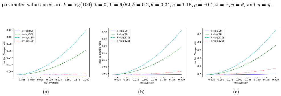
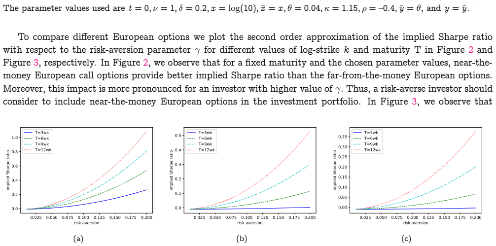
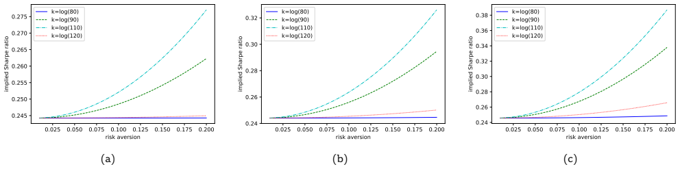
[Section 5, Figures 1-6] The numerical section provides no validation that the second-order expansion is accurate over the parameter ranges used: risk aversion γ from 0.025 to 0.2, option position ν up to 4, strikes from log(80) to log(120), and maturities from 3 to 12 weeks. No error bounds, convergence analysis, or comparison with a numerical PDE solution is given. In light of the sign and factor errors in Proposition 5, the plotted curves cannot be taken as reliable approximations to the true implied Sharpe ratio. Even after correcting the algebra, the paper needs to demonstrate, for at least one example, that the truncation error is small enough to justify the qualitative monotonicity claims.

minor comments (5)

[Section 2, Theorem 1] The proof of Theorem 1 is somewhat terse and contains a garbled display around the sign of ∂²_w V^M. The argument that V^M is strictly increasing in λ is correct in spirit, but the subsolution comparison is written in a way that is hard to follow; please rewrite the display cleanly.
[Section 2, Definition 3] Definition 3 requires the inequality V(t,s,w-νp,ν) ≥ U(w) to hold for all t∈[0,T] and all s>0, w,ν∈R. This is stronger than needed; the definition is only used at a fixed point (t,s,w,ν). Please restate the condition for the relevant point or clarify the intended domain.
[Section 5, Figures 2 and 5] The captions of Figures 2 and 5 state x = log(10), but the strikes shown range from log(80) to log(120); this appears to be a typo for x = log(100). Please correct the captions and check the actual parameter values used.
[Section 5, Heston and reciprocal Heston models] The notation in the SDEs is garbled in several places: for example, '∑1-ρ² t dB' should presumably be √(1-ρ²) dB_t^Y. Similar typographical issues appear in the reciprocal Heston model. These should be cleaned up for the final version.
[Section 4.1, Proposition 3] The formula for ψ2 in Proposition 3 contains a stray parenthesis and an ambiguously placed term involving (1/2λ²)²_{0,1}; the expression as printed is not well-formed. Please rewrite the formula with explicit brackets.

Circularity Check

0 steps flagged · score 0.0 of 10

No significant circularity: the implied Sharpe ratio is defined from the investor's value function, not fitted to data, and every approximation derives from the model PDEs.

full rationale

The central object, the implied Sharpe ratio, is introduced in Definition 3 as the unique positive solution of VM(t,w;Λ)=V(t,s,w−νp,ν), equivalently γνp+ψ=−(T−t)Λ²/2 in equation (10). The abstract's statement that the option with the highest implied Sharpe ratio improves expected utility the most is not a fitted prediction but an immediate consequence of the definition and the strict monotonicity of VM in λ, which the text explicitly acknowledges: 'From Definition 3, it is clear that a higher implied Sharpe ratio... will deliver a higher value to an investor.' No parameter is calibrated to market data: the option price p is computed under a chosen pricing measure, and ψ solves the HJB equation derived from the model. The asymptotic formulas in Propositions 3–5 are obtained by Taylor-expanding the PDE coefficients around (x̄,ȳ), an internal analytical approximation, not by postulating the desired comparative statics. The one self-citation, Lorig (2018), supplies the PDE expansion lemma (Lemma 2) used in the computations; this is a parameter-free commutation relation with stated smoothness assumptions, independent of the paper's target result, and is standard analytical machinery rather than an input equivalent to the conclusion. The reviewer's observation that Proposition 5's leading term should be |λ0| rather than λ0, and the possible extra factor 1/2 in Λ1, would be an internal consistency or algebraic correctness concern, not circularity: the object being expanded is still defined independently of the expansion. With no fitted input renamed as a prediction and no self-citation chain carrying the central claim, the derivation chain is self-contained and non-circular.

Assumptions & free parameters 0 free parameters · 4 assumptions · 0 invented entities

The central derivation is self-contained given the usual assumptions of stochastic control and the chosen pricing measure. The main additional assumptions are the exponential utility and the smoothness of coefficients. The numerical conclusions rest on the accuracy of the second-order truncation, which is not verified.

assumptions (4)

domain assumption The investor's utility is exponential: U(x) = -e^{-gamma x}/gamma for gamma > 0.
This choice makes the implied Sharpe ratio independent of initial wealth and permits the ansatz in Section 3. It is an assumption, not derived.
domain assumption The value function V is C^{1,2,2,2} and solves the HJB equation (6) with the candidate optimal feedback strategy.
Section 3 assumes smoothness to apply dynamic programming and derive the PDE for psi; standard verification arguments are not supplied.
domain assumption The coefficients in the local stochastic volatility model are C^2 (or analytic) in a neighborhood of the expansion point (xbar, ybar), so the Taylor-series expansion of the PDE coefficients is valid.
Section 4.1 assumes analyticity (or C^2) to justify the epsilon-expansion; this is a regularity requirement.
ad hoc to paper In the examples, the pricing measure is the minimal martingale measure (Omega=0 in (25)), which is the market's chosen pricing measure.
The implied Sharpe ratio depends on the option price p, and p depends on the chosen pricing measure. Setting Omega=0 in Section 5 is an arbitrary choice that affects all numerical results; the paper does not discuss sensitivity to Omega.

how reviews work

0 comments

Cite this review

Pith. "Pith review of The implied Sharpe ratio." pith.science (2026). https://pith.science/paper/FTUUDAC2

@misc{pith2026190804837,
  author       = {Pith},
  title        = {Pith review of: The implied Sharpe ratio},
  year         = {2026},
  howpublished = {\url{https://pith.science/paper/FTUUDAC2}},
  note         = {Machine review of arXiv:1908.04837}
}

read the original abstract

In an incomplete market, including liquidly-traded European options in an investment portfolio could potentially improve the expected terminal utility for a risk-averse investor. However, unlike the Sharpe ratio, which provides a concise measure of the relative investment attractiveness of different underlying risky assets, there is no such measure available to help investors choose among the different European options. We introduce a new concept -- the implied Sharpe ratio -- which allows investors to make such a comparison in an incomplete financial market. Specifically, when comparing various European options, it is the option with the highest implied Sharpe ratio that, if included in an investor's portfolio, will improve his expected utility the most. Through the method of Taylor series expansion of the state-dependent coefficients in a nonlinear partial differential equation, we also establish the behaviour of the implied Sharpe ratio with respect to an investor's risk-aversion parameter. In a series of numerical studies, we compare the investment attractiveness of different European options by studying their implied Sharpe ratio.

Figures

Figures reproduced from arXiv: 1908.04837 by the authors.

**Figure 1.** Implied Sharpe ratio for different values of log price (a) x = log(100) (b) x = log(110) (c) x = log(90). The parameter values used are k = log(100),t = 0, T = 6/52, δ = 0.2, θ = 0.04, κ = 1.15, ρ = –0.4, x¯ = x , y¯ = θ, and y = y¯. 0.025 0.050 0.075 0.100 0.125 0.150 0.175 0.200 risk aversion 0.00 0.02 0.04 0.06 0.08 0.10 0.12 implied Sharpe ratio k=log(80) k=log(90) k=log(110) k=log(120) (a) 0.025 0.050 0.075 0.1… view at source ↗

**Figure 2.** Relationship of the implied Sharpe ratio with respect to log-strike (a) T = 6/52 (b) T = 9/52 (c) T = 12/52. The parameter values used are t = 0, ν = 1, δ = 0.2, x = log(10), x¯ = x , θ = 0.04, κ = 1.15, ρ = –0.4, y¯ = θ, and y = y¯. To compare different European options we plot the second order approximation of the implied Sharpe ratio with respect to the risk-aversion parameter γ for different values of log-strike… view at source ↗

**Figure 3.** , respectively. In [PITH_FULL_IMAGE:figures/full_fig_p014_3.png] view at source ↗

Figures from the paper (3 more)

**Figure 4.** Figure 4: Implied Sharpe ratio for different values of log price (a) k = log(100), x = log(110) (b) k = log(100), x = log(100) (c) k = log(100), x = log(90). The parameter values used are t = 0, T = 0.25, µ = 0.05, a = 5.0, b = 0.04, κ = 0.01, ρ = 0.2, y¯ = 0.04, and y = y¯. 15 …

**Figure 5.** Figure 5: Relationship of the implied Sharpe ratio with respect to log-strike (a) T = 6/52 (b) T = 9/52 (c) T = 12/52. The parameter values used are t = 0, ν = 1, x = log(10), x¯ = x , µ = 0.05, a = 5.0, b = 0.04, κ = 0.01, ρ = 0.2, y¯ = 0.04, and y = y¯. We also compare differe…

**Figure 6.** Figure 6: Relationship of the implied Sharpe ratio with respect to maturity (a) k = log(100), x = log(110) (b) k = log(100), x = log(100) (c) k = log(100), x = log(90). The parameter values used are t = 0, ν = 1, x¯ = x , µ = 0.05, a = 5.0, b = 0.04, κ = 0.01, ρ = 0.2, y¯ = 0.04…

Discussion (0). Continue with ORCID to comment.

Reference graph

Works this paper leans on

16 extracted references · 15 canonical work pages

[1]

Carmona, R. (2008). Indifference pricing: theory and applications . Princeton University Press

work page 2008
[2]

Delbaen, F. and W. Schachermayer (2006). The mathematics of arbitrage . Springer Science & Business Media

work page 2006
[3]

Duffee, G. R. (2002). Term premia and interest rate forecasts in affine models. The Journal of Finance\/ 57\/ (1), 405--443

work page 2002
[4]

Gollier, and H

Eeckhoudt, L., C. Gollier, and H. Schlesinger (1995). The risk-averse (and prudent) newsboy. Management science\/ 41\/ (5), 786--794

work page 1995
[5]

Follmer, H. and M. Schweizer (1991). Hedging of contingent claims. Applied stochastic analysis\/ 5 , 389

work page 1991
[6]

Friedman, A. (2008). Partial differential equations of parabolic type . Courier Dover Publications

2008
[7]

Hodges, S. D. and A. Neuberger (1989). Optimal replication of contingent claims under transaction costs. The Review of Futures Markets\/ 8\/ (2), 222--239

work page 1989
[8]

Jensen, M. C. (1969). Risk, the pricing of capital assets, and the evaluation of investment portfolios. Journal of business\/ 42\/ (2), 167--247

work page 1969

Show all 16 references

[9]

Jewitt, I. (1987). Risk aversion and the choice between risky prospects: the preservation of comparative statics results. The Review of Economic Studies\/ 54\/ (1), 73--85

1987
[10]

Lorig, M. (2018). Indifference prices and implied volatilities. Mathematical Finance\/ 28\/ (1), 372--408

2018
[11]

Pagliarani, and A

Lorig, M., S. Pagliarani, and A. Pascucci (2015). Analytical expansions for parabolic equations. SIAM Journal on Applied Mathematics\/ 75\/ (2), 468--491

2015
[12]

Pagliarani, and A

Lorig, M., S. Pagliarani, and A. Pascucci (2017). Explicit implied volatilities for multifactor local-stochastic volatility models. Mathematical Finance\/ 27\/ (3), 926--960

2017
[13]

Merton, R. C. (1969). Lifetime portfolio selection under uncertainty: The continuous-time case. The Review of Economics and Statistics\/ , 247--257

1969
[14]

Pagliarani, S. and A. Pascucci (2012). Analytical approximation of the transition density in a local volatility model. Central European Journal of Mathematics\/ 10\/ (1), 250--270

2012
[15]

Pham, H. (2009). Continuous-time stochastic control and optimization with financial applications , Volume 61. Springer Science & Business Media

2009
[16]

Sharpe, W. F. (1966). Mutual fund performance. The Journal of Business\/ 39\/ (1), 119--138

1966

Pith tools

Reviewed August 14, 2026 · model on record in the stance chip above.

[1] [1]

Carmona, R. (2008). Indifference pricing: theory and applications . Princeton University Press

work page 2008

[2] [2]

Delbaen, F. and W. Schachermayer (2006). The mathematics of arbitrage . Springer Science & Business Media

work page 2006

[3] [3]

Duffee, G. R. (2002). Term premia and interest rate forecasts in affine models. The Journal of Finance\/ 57\/ (1), 405--443

work page 2002

[4] [4]

Gollier, and H

Eeckhoudt, L., C. Gollier, and H. Schlesinger (1995). The risk-averse (and prudent) newsboy. Management science\/ 41\/ (5), 786--794

work page 1995

[5] [5]

Follmer, H. and M. Schweizer (1991). Hedging of contingent claims. Applied stochastic analysis\/ 5 , 389

work page 1991

[6] [6]

Friedman, A. (2008). Partial differential equations of parabolic type . Courier Dover Publications

2008

[7] [7]

Hodges, S. D. and A. Neuberger (1989). Optimal replication of contingent claims under transaction costs. The Review of Futures Markets\/ 8\/ (2), 222--239

work page 1989

[8] [8]

Jensen, M. C. (1969). Risk, the pricing of capital assets, and the evaluation of investment portfolios. Journal of business\/ 42\/ (2), 167--247

work page 1969