REVIEW 4 major objections 5 minor 38 references
The Coulomb flux tube revisited
T0 review · 4 major / 5 minor · reviewed 2026-08-14 · deepseek-v4-flash
Pith's one-line read At finer lattice spacings, the Coulomb flux tube's transverse profile develops a power-law tail with exponent near 2, not the exponential decay seen on coarser lattices.
desk verdict New lattice data with a plausible but not yet demonstrated beta-dependence; the power-law tail claim needs a longer lever arm and a continuum extrapolation. read the letter →
The pith
A machine-rendered reading of the paper's core claim, the machinery that carries it, and where it could break.
The reading
What carries the argument
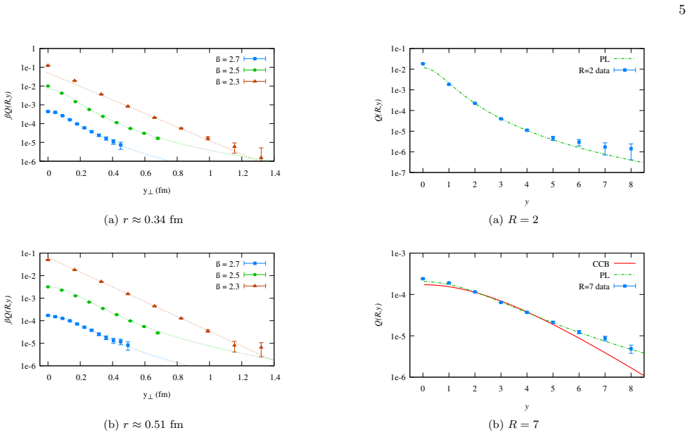
The central object is the lattice observable $Q_T(R,y)$, defined as a normalized correlation between two temporal Wilson lines of length $T$ and a plaquette probing the longitudinal chromoelectric field at transverse distance $y$ from the axis; $T=1$ gives the bare-state quantity of the earlier study. The argument runs through a comparison of two fitted models: the power-law shape $Q_{\mathrm{PL}}(R,y) = 16aR^2/(R^2+4y^2)^b$, where $b$ is the exponent of interest, and the exponential shape $Q_{\mathrm{CG}}(R,y) = \exp(-A-By)$. A third exponential-with-flattening model (CCB) is used for the coarsest lattice. The diagnostic is the large-$y$ behavior: exponential models fall faster than any power law, so the fitted exponent $b\approx 2$ at $\beta=2.7$, in agreement with the analytic prediction, is taken as evidence that the continuum profile is a power law.
What would settle it
A measurement of Q_{T=1}(R,y) at a finer lattice spacing (e.g., β = 2.9 or larger) that extends the transverse region to y*a ≳ 0.5 fm and shows the profile declining faster than any power law, or a fit whose exponent b moves away from 2 rather than toward it, would falsify the power-law claim. Equivalently, a continuum extrapolation of the fitted exponent from β = 2.5 and 2.7 that does not converge to b = 2 would do so.
Extended reading notes
Core claim
The central claim is that the normalized correlation $Q_{T=1}(R,y)$, which measures the longitudinal chromoelectric field component in the bare Coulomb state, changes its transverse falloff with the lattice coupling. At β = 2.3 the profile is well described by an exponential model for large quark separations; at β = 2.5 a power law with exponent $b \approx 2$ fits better than the exponential but with poor quality at large $R$; and at β = 2.7 the power law with $b \approx 2$ is clearly preferred for all $R$. The fitted exponent decreases from about 2.3–2.8 at small $R$ to about 2.1–2.2 at large $R$, converging to the value $b = 2$ predicted in the literature. The authors state that with increasing β it is likely that a genuine Coulomb flux tube with power-law falloff develops, and that the exponential result of the earlier single-β study was a finite-spacing effect.
Load-bearing premise
The load-bearing premise is that the transverse distances probed at β = 2.7 (y = 1 to 8 lattice units, i.e., 0.045 to 0.36 fm) are large enough to reveal the asymptotic power-law falloff, and that finite-volume and gauge-fixing systematics, which are not quantified, do not alter the qualitative comparison between exponential and power-law models.
Editorial extensions
If this is right
- If the power-law tail is genuine, the bare Coulomb flux tube has no finite width: its field extends to arbitrarily large transverse distances, consistent with the long-range nature of the Coulomb interaction.
- The earlier exponential result at β = 2.5 would be reinterpreted as a lattice-spacing artifact rather than a property of the continuum theory.
- The convergence of the fitted exponent toward b = 2 with decreasing lattice spacing supports the analytic prediction that the bare Coulomb state is not the same as the minimal Wilson state, and that the difference becomes visible only as the continuum is approached.
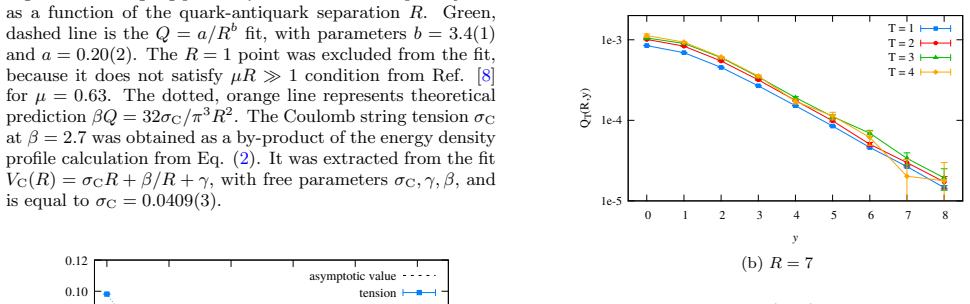
- The observed insensitivity of the profile shape to the Euclidean time T suggests that the bare state's flux-tube structure is already present at short times, and that larger volumes and finer lattices are needed to resolve its asymptotic form.
Reading between the lines
- One could test the power-law claim further by simulating at β ≈ 2.9 on a larger volume, where transverse distances beyond 0.5 fm become accessible; the fitted exponent should move toward 2 if the continuum tail is genuine.
- The same large-y analysis could be applied to other components of the energy density, such as the action density or the magnetic field, to check whether the power-law tail is a universal feature of the Coulomb flux tube or specific to the longitudinal electric field.
- A dedicated study of the near-axis region (small y), where the simple models fail, could separate a non-perturbative core from the asymptotic tail and reduce the fitting ambiguity that currently forces the exclusion of y = 0, 1, and sometimes 2.
- If the continuum Coulomb flux tube is indeed power-law, the 'string' picture of confining tubes is modified: the Coulomb part of the potential would receive contributions from transverse separations that grow with R, which might have observable consequences for the inter-quark potential at large distances.
Signed reviews
Editorial analysis
A structured set of objections, weighed in public.
Referee Report
Summary. The paper reports lattice measurements of the transverse profile Q_T=1(R,y) of the longitudinal chromoelectric field in Coulomb-gauge SU(2) Yang-Mills theory at beta=2.3, 2.5, and 2.7 on 32^4 lattices, extending the earlier work of Ref. [30] to larger statistics and additional couplings. The authors fit the profile with a power law Q_PL(R,y)=16aR^2/(R^2+4y^2)^b, an exponential Q_CG=exp(-A-By), and a modified exponential Q_CCB, and find that at beta=2.5 and 2.7 the large-y data favor a power law with fitted exponent b close to 2, in agreement with the analytic prediction of Ref. [8], while at beta=2.3 the profile is better described by an exponential. They also study the Euclidean-time dependence of Q_T and observe that the functional form does not visibly change with T. They conclude that, with increasing beta, a power-law Coulomb flux tube likely develops and that the profile may evolve from a Wilson-like to a Coulomb-like shape in the continuum limit, while cautioning that the small-y behavior is not reproduced by the power-law model. No continuum extrapolation is attempted, and finite-volume and gauge-fixing systematics are assumed not to affect the conclusion.
Significance. If correct, the result would overturn the exponential picture of the bare Coulomb flux tube reported in Ref. [30] and would provide lattice support for long-range Coulomb-gauge interactions and for the analytic prediction b about 2 of Ref. [8]. The paper's strengths are its transparent presentation: the complete Q_T=1 data set is shown in the appendix, fit parameters and chi2/dof values are tabulated for all R, jackknife errors are used, and the authors explicitly flag the fit-interval sensitivity and the lack of systematic-error estimates. These strengths make the measurement reproducible and the analysis auditable. The significance is, however, moderated by the fact that the central continuum statement rests on a short transverse lever arm (0.36 fm at beta=2.7) and on fits that require exclusion of small-y points; the result is therefore best read as a strong motivation for a dedicated continuum study rather than as an established continuum-limit result.
major comments (4)
- [Sec. III.A, Table IV] The beta=2.7 power-law claim relies on a very short lever arm: with a=0.045 fm the fit interval y in [1,8] covers only 0.045-0.36 fm, which is of the same order as the fitted exponential scales at beta=2.3 (Table III gives lambda about 1.3-2.1 lattice units, i.e. about 0.22-0.35 fm). The data therefore do not expose the asymptotic transverse tail, and a slowly decaying exponential or a transient cannot be excluded; a continuum-limit claim needs y_perp values well beyond the intrinsic scale.
- [Sec. III.A, Tables II and IV, Appendix A] The fitted exponent b is not robust against the choice of fit interval. Table IV states that b depends significantly on y_min and approaches 2 only as the low-y points are excluded, and at beta=2.5 the PL fits for R=5-8 have chi2/dof=10, 13, 19, 15 (Table II) despite the exclusion of y=0,1, and sometimes 2, admitted in Appendix A. This means the nominal b about 2 is controlled by a few large-y points; the paper should provide a y_min scan for fixed R and show that the power law is stable before claiming agreement with Ref. [8].
- [Sec. II.A] The assumption that finite-volume and gauge-fixing effects do not affect the main conclusion is load-bearing because the paper's conclusion is a statement about the continuum limit. The study uses one volume (32^4), one gauge-fixing criterion, and only three beta values, with no continuum extrapolation; the observed beta-dependence could include discretization or volume effects. At minimum the authors should estimate these systematics, for example with a second volume at beta=2.7 and a stricter gauge-fixing consistency check, and ideally add a fourth beta value or perform a continuum extrapolation of the fitted exponent b.
- [Sec. III.A, Fig. 4 and Table IV] At beta=2.7 the fitted exponent is strongly R-dependent for small separations (b=2.75(5) at R=1, 2.46(3) at R=2, decreasing to 2.09(3) at R=8), whereas the cited prediction of Ref. [8] is b about 2 independent of R. The text's statement that the profile falls as 1/y^4 in agreement with Ref. [8] is therefore only true at the largest R; the R-dependence of b needs to be addressed before the agreement is claimed.
minor comments (5)
- [Sec. IV] The sentence beginning with "with increasing beta the genuine, it is likely..." is ungrammatical, and "concussion" should be "conclusion"; please rewrite this passage.
- [Figure captions 9-11] "sperations" should be "separations" in the captions of Figs. 9, 10, and 11.
- [Sec. III.A and Fig. 3] The vertical-axis label in Fig. 3 is beta Q(R,y) while the text and fits use Q_T=1(R,y) and Q(R,y); please make the notation consistent and state which quantity is plotted.
- [Fig. 11 caption] The caption notes that the point (R=5, y=8, T=4) is negative but the text does not discuss this; because Q_T is a normalized expectation value, a negative value should be commented on, whether it is a statistical fluctuation, a subtraction artifact, or a finite-volume effect.
- [Sec. III.A, Eq. (8)] The sign of the -2 nu/lambda term in the CCB model is only explained in a footnote; please make the model definition self-contained and clarify the relation to the corresponding expression in Ref. [27].
Circularity Check
No circularity: the lattice fits are compared against an independent analytic prediction; interval choices are a data-analysis caveat, not a constructed equivalence.
full rationale
The paper's derivation chain is an empirical lattice measurement: define the correlation Q_T(R,y) in Eq. (3), compute it at beta = 2.3, 2.5, 2.7, fit competing models (CG, CCB, PL), and compare the fitted large-y power b with the analytic prediction b ~ 2 of Ref. [8]. No fitted parameter is defined in terms of the target conclusion. The PL form in Eq. (6) is an ansatz with free exponent b; the value b ~ 2 is an output of the fit, not imposed. The use of Ref. [8] is a genuine external benchmark: it is an analytic Dyson-Schwinger prediction made independently of these lattice data, so citing it is self-citation but not load-bearing circularity under rule 4. The admitted sensitivity of b to the fit interval (Tabs. II and IV) and the removal of small-y points (App. A) weaken the asymptotic claim and are correctness risks, but they are explicitly disclosed and do not make the comparison equivalent to its input. The absence of a continuum extrapolation and the Sec. II.A assumption that finite-volume and gauge-fixing errors do not affect the conclusion are also caveats, not circular reductions. Accordingly, the central result is self-contained against an independent theoretical prediction, and no circular step is exhibited.
Assumptions & free parameters
free parameters (5)
- PL amplitude a and exponent b (Eq. 6) =
Tables II, IV: e.g. b=2.114(4) at beta=2.5,R=2; b=2.75(5) at beta=2.7,R=1
- CG exponential parameters A, B (Eq. 7) =
Table I: e.g. A=6.58(2), B=0.554(8) at beta=2.5,R=7
- CCB parameters nu, lambda (Eq. 8) =
Table III: e.g. nu=2.587(4), lambda=1.973(3) at beta=2.3,R=7
- Coulomb string tension sigma_C at beta=2.7 =
0.0409(3) in lattice units
- Fit interval lower cutoff y_min =
1, 2, or 3 depending on R and model
assumptions (7)
- domain assumption Wilson action and heat-bath algorithm sample the correct SU(2) Yang-Mills ensemble.
- domain assumption Coulomb gauge fixing with Delta F < 10^-7 is sufficient and Gribov copies do not affect the result.
- domain assumption Q_T defined in Eq. (3) measures the x-component of the longitudinal chromoelectric field in the bare QQbar state.
- domain assumption Spatial links are close to identity in Coulomb gauge, so the Wilson loop can be approximated by two temporal Wilson lines.
- ad hoc to paper Finite lattice volume and gauge fixing quality do not affect the main conclusion.
- domain assumption Lattice spacings from Ref. [34] are correct for beta=2.3, 2.5, 2.7.
- domain assumption The asymptotic transverse falloff b=2 predicted in Ref. [8] is valid.
Cite this review
Pith. "Pith review of The Coulomb flux tube revisited." pith.science (2026). https://pith.science/paper/FYD3CSNP
@misc{pith2026190808874,
  author       = {Pith},
  title        = {Pith review of: The Coulomb flux tube revisited},
  year         = {2026},
  howpublished = {\url{https://pith.science/paper/FYD3CSNP}},
  note         = {Machine review of arXiv:1908.08874}
}
abstract
We perform $SU(2)$ Yang-Mills lattice simulation of the electric field distribution in the Coulomb gauge for different values of $\beta$ to further investigate the nature of the Coulomb flux tube.
Figures


Figures from the paper (7 more)



Reference graph
Works this paper leans on
-
[30]
with increased statistics. The concussion from [30] was that the Coulomb flux tube vanishes exponentially with the transverse distance, and has a width larger than the minimal flux tube. This is difficult to reconcile with theoretical prediction. We performed a somewhat differ- ent analysis of the same quantity by emphasizing large-y values. Furthermore by con...
-
[8]
P. O. Bowman and A. P. Szczepaniak, Phys. Rev. D70, 016002 (2004), arXiv:hep-ph/0403075 [hep-ph]
work page Pith review arXiv 2004
-
[1]
Renormalization-group Calculation of Color-Coulomb Potential
A. Cucchieri and D. Zwanziger, Phys. Rev. D65, 014002 (2001), arXiv:hep-th/0008248 [hep-th]
work page Pith review arXiv 2001
-
[2]
Confinement made simple in the Coulomb gauge
A. Cucchieri and D. Zwanziger, Lattice field theory. Pro- ceedings, 19th International Symposium, Lattice 2001, Berlin, Germany, August 19-24, 2001 , Nucl. Phys. Proc. Suppl. 106, 694 (2002), arXiv:hep-lat/0110189 [hep-lat]
work page Pith review arXiv 2002
-
[3]
A. P. Szczepaniak and E. S. Swanson, Phys. Rev. D65, 025012 (2002), arXiv:hep-ph/0107078 [hep-ph]
work page Pith review arXiv 2002
-
[4]
No confinement without Coulomb confinement
D. Zwanziger, Phys. Rev. Lett. 90, 102001 (2003), arXiv:hep-lat/0209105 [hep-lat]
work page Pith review arXiv 2003
-
[5]
Analytic calculation of color-Coulomb potential and color confinement
D. Zwanziger, Phys. Rev. D70, 094034 (2004), arXiv:hep-ph/0312254 [hep-ph]
work page Pith review arXiv 2004
-
[6]
Coulomb Energy, Vortices, and Confinement
J. Greensite and S. Olejnik, Phys. Rev. D67, 094503 (2003), arXiv:hep-lat/0302018 [hep-lat]
work page Pith review arXiv 2003
Show all 38 references
-
[7]
Cucchieri and D
A. Cucchieri and D. Zwanziger, Nuclear Physics B - Pro- ceedings Supplements 119, 727 (2003), proceedings of the XXth International Symposium on Lattice Field The- ory
2003
-
[9]
Nakagawa, A
Y. Nakagawa, A. Nakamura, T. Saito, H. Toki, and D. Zwanziger, Phys. Rev. D73, 094504 (2006), arXiv:hep-lat/0603010 [hep-lat]
2006 arXiv
-
[10]
Leder, H
M. Leder, H. Reinhardt, A. Weber, and J. M. Pawlowski, Phys. Rev. D86, 107702 (2012), arXiv:1105.0800 [hep- th]
2012 arXiv
-
[11]
Golterman, J
M. Golterman, J. Greensite, S. Peris, and A. P. Szczepa- niak, Phys. Rev. D85, 085016 (2012), arXiv:1201.4590 [hep-th]
2012 arXiv
-
[12]
Greensite and A
J. Greensite and A. P. Szczepaniak, Phys. Rev. D91, 034503 (2015), arXiv:1410.3525 [hep-lat]
2015 arXiv
-
[13]
Reinhardt, G
H. Reinhardt, G. Burgio, D. Campagnari, E. Ebadati, J. Heffner, M. Quandt, P. Vastag, and H. Vogt, 5th Win- ter Workshop on Non-Perturbative Quantum Field The- ory (WWNPQFT) Sophia-Antipolis, France, March 22- 24, 2017, Adv. High Energy Phys. 2018, 2312498 (2018), arXiv:1706.02...
2018 arXiv
-
[14]
Cooper and D
P. Cooper and D. Zwanziger, Phys. Rev. D98, 114006 (2018), arXiv:1803.06597 [hep-th]
2018 arXiv
-
[15]
V. N. Gribov, Nucl. Phys. B139, 1 (1978), [,1(1977)]
1978
-
[16]
Zwanziger, Nucl
D. Zwanziger, Nucl. Phys. B518, 237 (1998)
1998
-
[17]
Greensite, An introduction to the confinement problem, Lect
J. Greensite, An introduction to the confinement problem, Lect. Notes Phys. 821, 1 (2011)
2011
-
[18]
Fukugita and T
M. Fukugita and T. Niuya, Phys. Lett.132B, 374 (1983)
1983
-
[19]
J. W. Flower and S. W. Otto, Phys. Lett. 160B, 128 (1985)
1985
-
[20]
Wosiek and R
J. Wosiek and R. W. Haymaker, Phys. Rev. D36, 3297 (1987)
1987
-
[21]
J. B. Bronzan, Phys. Rev. D35, 3219 (1987)
1987
-
[22]
Di Giacomo, M
A. Di Giacomo, M. Maggiore, and S. Olejnik, Nucl. Phys. B347, 441 (1990)
1990
-
[23]
H. D. Trottier and R. M. Woloshyn, Phys. Rev. D48, 2290 (1993), arXiv:hep-lat/9303008 [hep-lat]
1993 arXiv
-
[24]
G. S. Bali, K. Schilling, and C. Schlichter, Phys. Rev. D51, 5165 (1995), arXiv:hep-lat/9409005 [hep-lat]
1995 arXiv
-
[25]
M. S. Cardaci, P. Cea, L. Cosmai, R. Falcone, and A. Papa, Phys. Rev. D83, 014502 (2011), arXiv:1011.5803 [hep-lat]
2011 arXiv
-
[26]
P. Cea, L. Cosmai, and A. Papa, Phys. Rev.D86, 054501 (2012), arXiv:1208.1362 [hep-lat]
2012 arXiv
-
[27]
Cardoso, M
N. Cardoso, M. Cardoso, and P. Bicudo, Phys. Rev. D88, 054504 (2013), arXiv:1302.3633 [hep-lat]
2013 arXiv
-
[28]
M. S. Lukashov and Yu. A. Simonov, Phys. Rev. D96, 076019 (2017), [Addendum: Phys. Rev.D98, 099903 (2018)], arXiv:1706.05712 [hep-ph]
2017 arXiv
-
[29]
Bicudo, N
P. Bicudo, N. Cardoso, and M. Cardoso, Phys. Rev. D 98, 114507 (2018)
2018
-
[31]
Chung and J
K. Chung and J. Greensite, Phys. Rev. D96, 034512 (2017), arXiv:1704.08995 [hep-lat]
2017 arXiv
-
[32]
Watson and H
P. Watson and H. Reinhardt, Phys. Rev. D82, 125010 (2010), arXiv:1007.2583 [hep-th]
2010 arXiv
-
[33]
Leder, J
M. Leder, J. M. Pawlowski, H. Reinhardt, and A. Weber, Phys. Rev. D83, 025010 (2011), arXiv:1006.5710 [hep- th]
2011 arXiv
-
[34]
K. G. Wilson, Phys. Rev. D 10, 2445 (1974)
1974
-
[35]
Bloch, A
J. Bloch, A. Cucchieri, K. Langfeld, and T. Mendes, Nuclear Physics B 687, 76 (2004)
2004
-
[36]
Creutz, Phys
M. Creutz, Phys. Rev. D 21, 2308 (1980)
1980
-
[37]
J. E. Mandula and M. Ogilvie, Physics Letters B 248, 156 (1990)
1990
-
[38]
Giusti, M
L. Giusti, M. L. Paciello, S. Petrarca, B. Tagli- enti, and C. Parrinello, International Jour- nal of Modern Physics A 16, 3487 (2001), https://doi.org/10.1142/S0217751X01004281
2001 doi
Reviewed August 14, 2026 · model on record in the stance chip above.
Discussion (0). Continue with ORCID to comment.