REVIEW 4 major objections 4 minor 1 cited by
Structural Parameters of the Thin Disk Population from Evolved Stars in Solar Neighborhood
T0 review · 4 major / 4 minor · reviewed 2026-08-10 · deepseek-v4-flash
Pith's one-line read Evolved stars in the solar neighborhood reveal that the thin disk's scale height rises from about 250 pc for the brightest to about 430 pc for the faintest.
desk verdict A useful Gaia DR3 extension of the known scale-height trend for evolved stars, but the faintest bins are weakly constrained by the survey volume and the quoted errors are too small. read the letter →
The pith
A machine-rendered reading of the paper's core claim, the machinery that carries it, and where it could break.
The reading
What carries the argument
The load-bearing object is the single-component vertical density law $D(z) = n \exp(-|z+z_0|/H)$, applied to evolved stars as tracers. Because the sample is confined to 1 kpc, the radial term of the double-exponential disk cannot be constrained, so the fit isolates the vertical scale height $H$. The analysis pipeline is built on three choices: a strict relative parallax cut ($\sigma_\varpi/\varpi \le 0.02$) to define reliable distances, a completeness cut per magnitude bin derived from apparent-magnitude limits, and a division into 36 equal-area Galactic fields and five absolute-magnitude intervals. The scale height is then read off as the best-fit $H$ by chi-square minimization over $100 < H < 1000$ pc for each of the 180 profiles. The mass interpretation is carried by stellar evolution tracks, which convert absolute magnitude into progenitor mass and main-sequence lifetime.
What would settle it
Rebuild the same 180 density profiles in the faintest magnitude bin ($3 < M_{\rm G} \le 4$) with a two-component thin-plus-thick disk model: if the recovered thin-disk scale height drops toward 300 pc or the bright-to-faint increasing trend disappears, the claimed gradient is contamination rather than a memory of progenitor scale heights. Alternatively, measure the vertical velocity dispersion of stars in the brightest and faintest bins with Gaia radial velocities; a genuine scale-height rise from ~250 to ~430 pc should be accompanied by a rise in vertical velocity dispersion of roughly a factor of two.
Extended reading notes
Core claim
The paper's central claim is that the vertical density profile of evolved stars in the solar neighborhood is an exponential with a scale height that grows linearly with absolute magnitude: $H_{\rm North} = 37.1 \times M_{\rm G} + 276$ pc and $H_{\rm South} = 43.4 \times M_{\rm G} + 288$ pc ($R^2 \approx 0.97$). The authors establish this by splitting 671,600 Gaia DR3 evolved stars with relative parallax errors below 0.02 into 36 Galactic fields and five one-magnitude bins, building 180 space-density profiles, and fitting each with the single-component law $D(z) = n \exp(-|z+z_0|/H)$. They show the fitted space densities match the solar-neighborhood luminosity function, and a Monte Carlo check in one field indicates thin-disk scale heights are only mildly affected by thick-disk and halo contamination. The resulting gradient, from about 250 pc to about 430 pc, is interpreted as the memory of the scale height of the main-sequence progenitors: brighter evolved stars come from early-type stars with short scale heights, fainter ones from intermediate-type stars with large scale heights.
Load-bearing premise
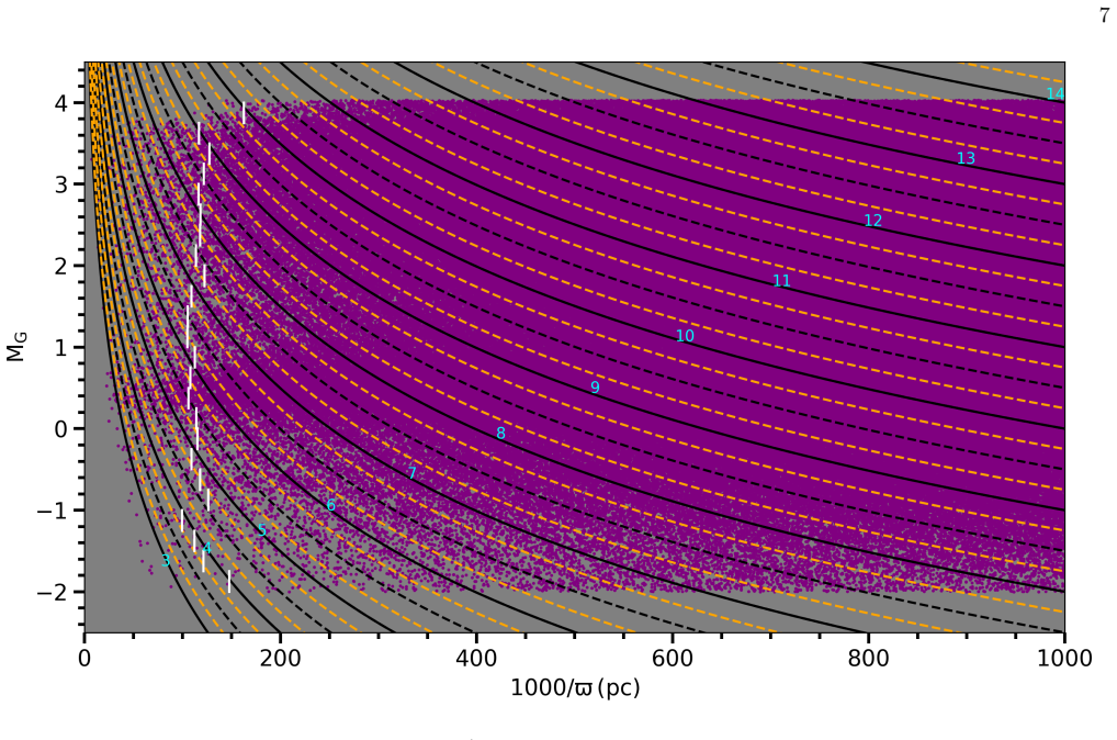
The analysis assumes a single exponential density profile dominated by thin-disk stars, and for the lowest-latitude fields the observed lines of sight reach only about 425 to 770 pc above the plane — less than three scale heights for the largest $H$ values — so the fits are constrained by the inner part of the profile rather than by the full vertical structure.
Editorial extensions
If this is right
- Any thin-disk model that uses one global scale height (e.g., 300 pc) is incomplete; the data imply a magnitude-dependent scale height that must be folded into star-count and kinematic models.
- Red clump stars, with $H = 295 \pm 10$ pc, can serve as a robust vertical-distance anchor for the solar neighborhood, useful for calibrating other distance indicators.
- The scale-height gradient implies a vertical mass stratification: fainter, lower-mass evolved stars are found at larger heights, which affects the interpretation of any magnitude-limited sample of giants.
- If the trend continues beyond $M_{\rm G} = 4$, then even fainter evolved stars (such as white-dwarf progenitors) would imply larger scale heights, which would alter estimates of the local dark-matter density derived from vertical Jeans modeling.
- The agreement of fitted space densities with the literature luminosity function suggests the gradient is not a fitting artifact, so the result can be used to test models of disk heating and star formation history.
Reading between the lines
- The linear relations could be pushed further: combining the fitted $H(M_{\rm G})$ with main-sequence lifetimes and birth positions predicts a present-day vertical velocity dispersion gradient of roughly 15 to 30 km/s across the magnitude range, which is testable with Gaia radial velocities.
- The unexplained 12 pc north–south zero-point offset might be a real large-scale asymmetry (a warp or a tilt of the Sun's height relative to the midplane) or a systematic in the dust correction; a larger sample that includes fields below $|b|=25^\circ$, where the profile reaches several scale heights, would distinguish these.
- The memory interpretation implies that in galaxies seen edge-on, the thickness of the red giant/red clump layer should correlate with the stellar mass of the population, offering a way to test the result outside the Milky Way.
- The single-exponential assumption could be relaxed by fitting a ${\rm sech}^2$ or two-component law; the paper's trend would be strengthened if the faintest bins still prefer large scale heights under those models.
Signed reviews
Editorial analysis
A structured set of objections, weighed in public.
Referee Report
Summary. The paper uses Gaia DR3 astrometry and photometry to select 671,600 evolved stars (after a relative-parallax cut of 0.02) within a 1 kpc heliocentric volume, dereddens them with the Schlafly & Finkbeiner (2011) dust map, divides the sky into 36 Galactic fields and the absolute-magnitude range -1 < MG ≤ 4 into five 1-mag bins, and fits a single-component exponential density law (Eq. 3) to the resulting space-density profiles. The reported result is that the thin-disk scale height increases from roughly 250 pc in the brightest bin to roughly 430 pc in the faintest bin, with median relations H_North = 37.1 MG + 276 and H_South = 43.4 MG + 288 (Eq. 10), and a red-clump scale height of 295 ± 10 pc. The authors interpret this as evidence that evolved stars retain the vertical scale height of their main-sequence progenitors.
Significance. If the quantitative result is robust, the paper provides a clean, parallax-based measurement of how the thin-disk scale height varies with the absolute magnitude of evolved stars, connecting the vertical structure of the disk to stellar evolution. Strengths of the paper include the large Gaia-based sample, the explicit treatment of extinction and completeness, the use of the authors' own Monte Carlo contamination check (albeit in only one field/bin), and the agreement of the recovered space densities with the Gaia Collaboration (2021b) luminosity function. The absence of circularity in the analysis is notable: all quantities (n, H, and the linear fits) are estimated from the data and compared with independent literature values. However, the central quantitative claim — the slope of Eq. 10 and the largest H values of 400–600 pc — rests on fits to density profiles that sample only a small fraction of the fitted exponential, as detailed in the major comments.
major comments (4)
- [§3.5 and Table A1] The paper's own criterion for reliable scale-height determination — that the data must extend to 3–5 scale heights — is violated for the very fields and magnitude bins that produce the largest H values. For fields with 25° < |b| ≤ 50° and d ≤ 1 kpc, the maximum vertical height is only z_max = 425–770 pc. For H values of 400–600 pc reported in the faintest bins (e.g., Table A1 fields #01, #19, #20, #14, #15, #36), the density profile samples only approximately 0.7–1.9 H. Over such a short baseline the single exponential fit is strongly degenerate between the local density n and H, so the large H values in these bins, and consequently the slope of Eq. 10, are not securely constrained. The authors should either restrict the analysis to fields where the baseline is at least 3 H or demonstrate, with mock catalogues, that H is recovered without bias from the short-baseline profiles.
- [Table A1 and Section 3.5] Several quoted uncertainties are implausibly small given the coarse 200 pc distance binning and the short vertical baseline; for example H = 405 ± 1 pc (field #06, 2 < MG ≤ 3), H = 344 ± 3 pc (field #03, 3 < MG ≤ 4), and H = 450 ± 17 pc (field #02, 2 < MG ≤ 3). These errors appear to reflect only the 1 pc step of the grid search and not the covariance between n and H, the finite bin-width effects, or the systematic uncertainties in the extinction and parallax zero point. The error-weighted mean quoted for the red clump (H = 295 ± 10 pc) and the comparison with literature values in Section 4 are therefore likely over-optimistic; the authors should propagate more realistic uncertainties, e.g., via bootstrap or profile likelihood, before the linear relations in Eq. 10 can be taken at face value.
- [Section 4, Monte Carlo test] The Monte Carlo contamination test is performed only for field #01 in the absolute-magnitude bin 0 < MG ≤ 1, where H ≈ 300 pc and z_max/H ≈ 2.5. The faintest bins (2 < MG ≤ 3 and 3 < MG ≤ 4) have larger fitted H values and are exactly the cases where a contaminating thicker component (thick disk or halo) would bias the single-exponential fit most strongly. The claim that the thin-disk scale height is 'minimally affected' by other Galactic populations is therefore not demonstrated for the bins that drive the largest H values and the slope of Eq. 10. The authors should run the same Monte Carlo exercise for all five magnitude bins, or at least for the two faintest ones, and report how the recovered H changes when a thick-disk component with the assumed parameters is added.
- [Section 3.3, completeness definition] The completeness threshold is defined by identifying the 'initial 0.5% slice of the G-band apparent magnitude distribution within each absolute magnitude bin' (Section 3.3). This is an ad hoc choice, and it is not demonstrated that the resulting distance cuts remove the incompleteness bias in the density profiles. Because the faintest magnitude bins are the ones most affected by incompleteness at large distances, and because those bins dominate the largest H values, the sensitivity of the fitted H to the percentile choice (say 0.1% versus 1%) should be quantified; if H changes appreciably, the completeness criterion is load-bearing for the central claim.
minor comments (4)
- [Section 4, Figure 8 caption] The text refers to the 'CDM' when the intended term is 'CMD'; this typo appears in the sentence describing Figure 8 and should be corrected.
- [Introduction, literature survey] The description of the Two Micron All Sky Survey is given as 'Two Micron Sky Survey'; the correct full name is 'Two Micron All Sky Survey'.
- [Equation 8 and Section 3.4] The volume element in Eq. 8 is the solid-angle volume between distances d1 and d2, but the paper does not state how the field size □ is computed for the curved sky regions defined in Section 3.5; a short clarification would help readers reproduce the density profiles.
- [Table A1 and Table 1] The notation for magnitude intervals is inconsistent between the text ('-1 < MG ≤ 0') and the table headers ('(-1, 0]'), and the same field numbering is used in both tables; a consistent notation and a note in the caption would improve readability.
Circularity Check
No significant circularity: the scale heights are fitted directly from Gaia density profiles and checked against independent literature values; self-citations are contextual rather than load-bearing.
full rationale
The paper's central claims are the fitted thin-disk scale heights for five absolute-magnitude bins and the increasing trend summarized by Eq. 10. These are not derived from a fitted parameter renamed as a prediction. The density law D(z) = n exp(-|z+z0|/H) (Eq. 3) is a standard model assumption; H and n are free parameters determined for each star field and magnitude bin by chi-square minimization against densities computed from star counts (Eqs. 7-9). No fitted value is then used to generate the same or a closely related quantity by construction. Equation 10 is a least-squares summary of the medians of these independently fitted H values, so it is descriptive and could have come out flat; it is not forced by the fitting procedure. The paper also benchmarks its results externally: space densities are compared with the Gaia Collaboration et al. 2021b luminosity function, the red-clump scale height (295 +/- 10 pc) is compared with the independent APOGEE-based value of Bovy et al. 2016b, and the overall trend is compared with earlier photometric determinations. The many self-citations (Bilir et al., Karaali et al., Ak et al., etc.) provide context and, in the Monte Carlo test, parameter ranges for the thick disk and halo; these do not enter the definition of the thin-disk H fit or the Eq. 10 relation, and the Monte Carlo test is only an auxiliary robustness check on one field. Concerns about the faint-bin scale heights being weakly constrained because the survey reaches only about 1-1.5 H in the low-latitude fields are legitimate robustness or correctness concerns, but they are not circularity: the fit is still an honest fit to the data, not an input recycled as an output.
Assumptions & free parameters
free parameters (4)
- H (scale height) =
200 to 600 pc per field/magnitude bin
- n (local space density) =
10^(D*−10) per field/magnitude bin
- Slope and intercept of H(MG) relations =
37.1, 276 (north); 43.4, 288 (south)
- Completeness threshold percentile =
0.5%
assumptions (5)
- domain assumption Vertical density profile follows a single exponential D(z) = n exp(−|z + z0| / H).
- domain assumption Evolved stars can be isolated by the CMD region (0.8 < (GBP−GRP)0 < 2.2, −3 < MG < 4) with negligible main-sequence contamination.
- domain assumption Stars within 1 kpc are predominantly thin-disk members; thick disk and halo contributions are small.
- domain assumption The Schlafly and Finkbeiner (2011) dust map with Bahcall and Soneira distance scaling and the Cardelli et al. (1989) extinction curve correctly deredden Gaia photometry.
- ad hoc to paper The 0.5% slice of the apparent magnitude distribution identifies the onset of incompleteness.
Cite this review
Pith. "Pith review of Structural Parameters of the Thin Disk Population from Evolved Stars in Solar Neighborhood." pith.science (2026). https://pith.science/paper/FZB36I7C
@misc{pith2026250104079,
  author       = {Pith},
  title        = {Pith review of: Structural Parameters of the Thin Disk Population from Evolved Stars in Solar Neighborhood},
  year         = {2026},
  howpublished = {\url{https://pith.science/paper/FZB36I7C}},
  note         = {Machine review of arXiv:2501.04079}
}
abstract
This study investigates the structural parameters of the thin-disk population by analyzing the spatial distribution of evolved stars in the solar neighbourhood. From the $\it Gaia$ Data Release 3 database, about 39.1 million stars within 1 kpc and with relative parallax errors $\sigma_{\varpi}/\varpi\leq 0.10$ were selected. The photometric data was corrected for extinction using a Galactic dust map. The sample was refined by considering the color-magnitude region $M_{\rm G}\times (G_{\rm BP}-G_{\rm RP})_0$ associated with evolved stars, applying a stricter parallax error limit of $\sigma_{\varpi}/\varpi\leq 0.02$, and yielding 671,600 stars. The star sample was divided into 36 regions based on their Galactic coordinates, with evolved stars in the absolute magnitude range of $-1< M_{\rm G}~{\rm (mag)}\leq 4$ further split into five one-unit magnitude intervals. This led to 180 subgroups whose space density profiles were modelled using a single-component Galaxy model. The analysis shows that the space densities are in agreement with the literature and that the scale heights vary with $200<H~{\rm (pc)}<600$ interval to their absolute magnitudes. Red clump stars in the solar neighbourhood were also estimated to have a scale height of $295\pm10$ pc. These findings indicate that evolved stars with bright absolute magnitudes originate from the evolution of the early spectral-type stars with short scale height, while fainter ones come from the evolution of the intermediate spectral-type stars with large scale height, suggesting variations in scale height reflect the contribution of Galactic evolution processes.
Figures


Figures from the paper (5 more)


Forward citations
Cited by 1 Pith paper
-
Kings of the Milky Way: A Homogeneous Gaia DR3 Analysis of King Open Clusters and the Galactic Disc Metallicity Gradient
A homogeneous Gaia DR3 re-analysis of all 27 King open clusters gives consistent parameters and a metallicity gradient of about -0.06 dex/kpc, but the King-only slope is not statistically significant as printed.
Reference graph
Works this paper leans on
-
[1]
2007a, Astronomische Nachrichten, 328, 169, doi: 10.1002/asna.200610709
Ak, S., Bilir, S., Karaali, S., & Buser, R. 2007a, Astronomische Nachrichten, 328, 169, doi: 10.1002/asna.200610709
-
[2]
2007b, NewA, 12, 605, doi: 10.1016/j.newast.2007.04.005 Astropy Collaboration, Robitaille, T
Ak, S., Bilir, S., Karaali, S., Buser, R., & Cabrera-Lavers, A. 2007b, NewA, 12, 605, doi: 10.1016/j.newast.2007.04.005 Astropy Collaboration, Robitaille, T. P., Tollerud, E. J., et al. 2013, A&A, 558, A33, doi: 10.1051/0004-6361/201322068 Astropy Collaboration, Price-Whelan, A. M., Sip˝ ocz, B. M., et al. 2018, AJ, 156, 123, doi: 10.3847/1538-3881/aabc4f...
-
[3]
Bahcall, J. N., & Soneira, R. M. 1980, ApJS, 44, 73, doi: 10.1086/190685
doi:10.1086/190685 1980
-
[4]
2008a, PASA, 25, 69, doi: 10.1071/AS07026
Bilir, S., Cabrera-Lavers, A., Karaali, S., et al. 2008a, PASA, 25, 69, doi: 10.1071/AS07026
-
[5]
2009, MNRAS, 396, 1589, doi: 10.1111/j.1365-2966.2009.14816.x —
Bilir, S., Karaali, S., Ak, S., et al. 2009, MNRAS, 396, 1589, doi: 10.1111/j.1365-2966.2009.14816.x —. 2008b, MNRAS, 390, 1569, doi: 10.1111/j.1365-2966.2008.13839.x
arXiv 2009
-
[6]
2006a, NewA, 12, 234, doi: 10.1016/j.newast.2006.10.001
Bilir, S., Karaali, S., Ak, S., Yaz, E., & Hamzao˘ glu, E. 2006a, NewA, 12, 234, doi: 10.1016/j.newast.2006.10.001
-
[7]
2006b, MNRAS, 366, 1295, doi: 10.1111/j.1365-2966.2006.09891.x
Bilir, S., Karaali, S., & Gilmore, G. 2006b, MNRAS, 366, 1295, doi: 10.1111/j.1365-2966.2006.09891.x
arXiv 2006
-
[8]
Bilir, S., Karaali, S., G¨ uver, T., Karata¸ s, Y., & Ak, S. G. 2006c, Astronomische Nachrichten, 327, 72, doi: 10.1002/asna.200510480
Show all 57 references
-
[9]
2005, Astronomische Nachrichten, 326, 321, doi: 10.1002/asna.200510358
Bilir, S., Karaali, S., & Tun¸ cel, S. 2005, Astronomische Nachrichten, 326, 321, doi: 10.1002/asna.200510358
2005 doi
-
[10]
1998, Galactic Astronomy
Binney, J., & Merrifield, M. 1998, Galactic Astronomy
1998
-
[11]
Finkbeiner, D. P. 2016a, ApJ, 818, 130, doi: 10.3847/0004-637X/818/2/130
-
[12]
F., et al
Bovy, J., Rix, H.-W., Schlafly, E. F., et al. 2016b, ApJ, 823, 30, doi: 10.3847/0004-637X/823/1/30 4 https://www.cosmos.esa.int/gaia 5 https://www.cosmos.esa.int/web/gaia/dpac/consortium
-
[13]
2012, MNRAS, 427, 127, doi: 10.1111/j.1365-2966.2012.21948.x
Bressan, A., Marigo, P., Girardi, L., et al. 2012, MNRAS, 427, 127, doi: 10.1111/j.1365-2966.2012.21948.x
2012
-
[14]
1998, A&A, 331, 934 —
Buser, R., Rong, J., & Karaali, S. 1998, A&A, 331, 934 —. 1999, A&A, 348, 98
1998
-
[15]
2007, A&A, 464, 565, doi: 10.1051/0004-6361:20066475
Cabrera-Lavers, A., Bilir, S., Ak, S., Yaz, E., & L´ opez-Corredoira, M. 2007, A&A, 464, 565, doi: 10.1051/0004-6361:20066475
2007 doi
-
[16]
2023, AJ, 165, 163, doi: 10.3847/1538-3881/acbead
Canbay, R., Bilir, S., ¨Ozd¨ onmez, A., & Ak, T. 2023, AJ, 165, 163, doi: 10.3847/1538-3881/acbead
2023 doi
-
[17]
A., Clayton, G
Cardelli, J. A., Clayton, G. C., & Mathis, J. S. 1989, ApJ, 345, 245, doi: 10.1086/167900
1989 doi
-
[18]
R., et al
Castro-Ginard, A., Penoyre, Z., Casey, A. R., et al. 2024, A&A, 688, A1, doi: 10.1051/0004-6361/202450172
2024 doi
-
[19]
A., et al
Chen, B., Stoughton, C., Smith, J. A., et al. 2001, ApJ, 553, 184, doi: 10.1086/320647
2001 doi
-
[20]
2015, MNRAS, 452, 1068, doi: 10.1093/mnras/stv1281 Chrob´ akov´ a,ˇZ., Nagy, R., & L´ opez-Corredoira, M
Chen, Y., Bressan, A., Girardi, L., et al. 2015, MNRAS, 452, 1068, doi: 10.1093/mnras/stv1281 Chrob´ akov´ a,ˇZ., Nagy, R., & L´ opez-Corredoira, M. 2020, A&A, 637, A96, doi: 10.1051/0004-6361/201937289
2015 doi
-
[21]
1995, ApJ, 444, 874, doi: 10.1086/175659
Cohen, M. 1995, ApJ, 444, 874, doi: 10.1086/175659
1995 doi
-
[22]
2003, A&A, 407, 541, doi: 10.1051/0004-6361:20030532
Du, C., Zhou, X., Ma, J., et al. 2003, A&A, 407, 541, doi: 10.1051/0004-6361:20030532
2003 doi
-
[23]
2024, Physics and Astronomy Reports, 2, 41, doi: 10.26650/PAR.2024.00001
Eker, Z., Soydugan, F., & Bilir, S. 2024, Physics and Astronomy Reports, 2, 41, doi: 10.26650/PAR.2024.00001
2024
-
[24]
2015, AJ, 149, 131, doi: 10.1088/0004-6256/149/4/131
Eker, Z., Soydugan, F., Soydugan, E., et al. 2015, AJ, 149, 131, doi: 10.1088/0004-6256/149/4/131
2015 doi
-
[25]
2018, MNRAS, 479, 5491, doi: 10.1093/mnras/sty1834
Eker, Z., Bakı¸ s, V., Bilir, S., et al. 2018, MNRAS, 479, 5491, doi: 10.1093/mnras/sty1834
2018 doi
-
[26]
2020, MNRAS, 496, 3887, doi: 10.1093/mnras/staa1659
Eker, Z., Soydugan, F., Bilir, S., et al. 2020, MNRAS, 496, 3887, doi: 10.1093/mnras/staa1659
2020 doi
-
[27]
1987, A&AS, 69, 33 Gaia Collaboration, Prusti, T., de Bruijne, J
Fenkart, R., & Karaali, S. 1987, A&AS, 69, 33 Gaia Collaboration, Prusti, T., de Bruijne, J. H. J., et al. 2016, A&A, 595, A1, doi: 10.1051/0004-6361/201629272 Gaia Collaboration, Babusiaux, C., van Leeuwen, F., et al. 2018, A&A, 616, A10, doi: 10.1051/0004-6361/201832843 Gaia...
1987 doi
-
[28]
1983, MNRAS, 202, 1025, doi: 10.1093/mnras/202.4.1025
Gilmore, G., & Reid, N. 1983, MNRAS, 202, 1025, doi: 10.1093/mnras/202.4.1025
1983 doi
-
[29]
2023, AJ, 166, 263, doi: 10.3847/1538-3881/ad08b0
Gokmen, S., Eker, Z., Yontan, T., et al. 2023, AJ, 166, 263, doi: 10.3847/1538-3881/ad08b0
2023 doi
-
[30]
Warren, S. J. 1996, ApJS, 104, 185, doi: 10.1086/192297
1996 doi
-
[31]
L., Garzon, F., Mahoney, T., & Calbet, X
Hammersley, P. L., Garzon, F., Mahoney, T., & Calbet, X. 1995, MNRAS, 273, 206, doi: 10.1093/mnras/273.1.206
1995 doi
-
[32]
R., Millman, K
Harris, C. R., Millman, K. J., van der Walt, S. J., et al. 2020, Nature, 585, 357, doi: 10.1038/s41586-020-2649-2
2020 doi
-
[33]
Hawkins, M. R. S. 1988, MNRAS, 234, 533, doi: 10.1093/mnras/234.3.533
1988 doi
-
[34]
W., Trenti, M., Clarkson, W., et al
Holwerda, B. W., Trenti, M., Clarkson, W., et al. 2014, ApJ, 788, 77, doi: 10.1088/0004-637X/788/1/77
2014 doi
-
[35]
Hunter, J. D. 2007, Computing in Science & Engineering, 9, 90, doi: 10.1109/MCSE.2007.55 Juri´ c, M., Ivezi´ c,ˇZ., Brooks, A., et al. 2008, ApJ, 673, 864, doi: 10.1086/523619
2007 doi
-
[36]
G., Bilir, S., Karata¸ s, Y., & Gilmore, G
Karaali, S., Ak, S. G., Bilir, S., Karata¸ s, Y., & Gilmore, G. 2003, MNRAS, 343, 1013, doi: 10.1046/j.1365-8711.2003.06743.x
2003
-
[37]
2004, MNRAS, 355, 307, doi: 10.1111/j.1365-2966.2004.08319.x
Karaali, S., Bilir, S., & Hamzaoˇ glu, E. 2004, MNRAS, 355, 307, doi: 10.1111/j.1365-2966.2004.08319.x
2004
-
[38]
2005, PASA, 22, 24, doi: 10.1071/AS04034
Karaali, S., Bilir, S., & Tun¸ cel, S. 2005, PASA, 22, 24, doi: 10.1071/AS04034
2005 doi
-
[39]
2007, PASA, 24, 208, doi: 10.1071/AS07006
Karaali, S., Bilir, S., Yaz, E., Hamzao˘ glu, E., & Buser, R. 2007, PASA, 24, 208, doi: 10.1071/AS07006
2007 doi
-
[40]
2009, Ap&SS, 324, 23, doi: 10.1007/s10509-009-0149-9
Karaali, S., Hamzao˘ glu, E., & Bilir, S. 2009, Ap&SS, 324, 23, doi: 10.1007/s10509-009-0149-9
2009 doi
-
[41]
L., & Zhu, Z
Kong, D. L., & Zhu, Z. 2008, Acta Astronomica Sinica, 49, 224
2008
-
[42]
2021, A&A, 649, A4, doi: 10.1051/0004-6361/202039653
Lindegren, L., Bastian, U., Biermann, M., et al. 2021, A&A, 649, A4, doi: 10.1051/0004-6361/202039653
2021 doi
-
[43]
Majewski, S. R. 1993, ARA&A, 31, 575, doi: 10.1146/annurev.aa.31.090193.003043
1993
-
[44]
2006, A&A, 453, 635, doi: 10.1051/0004-6361:20053842
Picaud, S. 2006, A&A, 453, 635, doi: 10.1051/0004-6361:20053842
2006 doi
- [45]
-
[46]
Peiris, H. V. 2000, ApJ, 544, 811, doi: 10.1086/317241
2000 doi
-
[47]
C., Burgasser, A., et al
Pirzkal, N., Sahu, K. C., Burgasser, A., et al. 2005, ApJ, 622, 319, doi: 10.1086/427896
2005 doi
-
[48]
F., & Finkbeiner, D
Schlafly, E. F., & Finkbeiner, D. P. 2011, ApJ, 737, 103, doi: 10.1088/0004-637X/737/2/103
2011 doi
-
[49]
H., Majewski, S
Siegel, M. H., Majewski, S. R., Reid, I. N., & Thompson, I. B. 2002, ApJ, 578, 151, doi: 10.1086/342469
2002 doi
-
[50]
F., Cutri, R
Skrutskie, M. F., Cutri, R. M., Stiening, R., et al. 2006, AJ, 131, 1163, doi: 10.1086/498708
2006 doi
-
[51]
2014, MNRAS, 445, 4287, doi: 10.1093/mnras/stu2029
Tang, J., Bressan, A., Rosenfield, P., et al. 2014, MNRAS, 445, 4287, doi: 10.1093/mnras/stu2029
2014 doi
-
[52]
2023, Physics and Astronomy Reports, 1, 1, doi: 10.26650/PAR.2023.00001 Van Rossum, G., & Drake, F
Tasdemir, S., & Yontan, T. 2023, Physics and Astronomy Reports, 1, 1, doi: 10.26650/PAR.2023.00001 Van Rossum, G., & Drake, F. L. 2009, Python 3 Reference Manual (Scotts Valley, CA: CreateSpace)
2023
-
[53]
2018, MNRAS, 478, 3367, doi: 10.1093/mnras/sty1058
Wang, H.-F., Liu, C., Xu, Y., Wan, J.-C., & Deng, L. 2018, MNRAS, 478, 3367, doi: 10.1093/mnras/sty1058
2018 doi
-
[54]
2010, NewA, 15, 234, doi: 10.1016/j.newast.2009.07.010 Yaz G¨ ok¸ ce, E., Karaali, S., Duran, S ¸., et al
Yaz, E., & Karaali, S. 2010, NewA, 15, 234, doi: 10.1016/j.newast.2009.07.010 Yaz G¨ ok¸ ce, E., Karaali, S., Duran, S ¸., et al. 2015, PASA, 32, e012, doi: 10.1017/pasa.2015.12
2010 doi
- [55]
-
[56]
G., Adelman, J., Anderson, John E., J., et al
York, D. G., Adelman, J., Anderson, John E., J., et al. 2000, AJ, 120, 1579, doi: 10.1086/301513
2000 doi
-
[57]
2021, ApJ, 922, 80, doi: 10.3847/1538-4357/ac1e91 14 APPENDIX A
Yu, Y., Wang, H.-F., Cui, W.-Y., et al. 2021, ApJ, 922, 80, doi: 10.3847/1538-4357/ac1e91 14 APPENDIX A. ADDITIONAL FIGURES AND TABLES T able A1. Galaxy model parameters estimated for five different abso- lute magnitude intervals in the 36-star fields. 0◦ < l≤ 60◦, 25◦ < b≤ 50...
2021 doi
Reviewed August 10, 2026 · model on record in the stance chip above.
Discussion (0). Continue with ORCID to comment.