REVIEW 1 major objections 4 minor 4 references
A Multinomial Probit Model for Asymmetric Choice Responses
T0 review · 1 major / 4 minor · reviewed 2026-08-15 · deepseek-v4-flash
Pith's one-line read A skewed multinomial probit model allows choice probabilities to respond asymmetrically to covariate changes, and the paper shows it is identified and estimable.
desk verdict A genuinely useful reparameterization for skewed multinomial probit with a workable sampler, but identification is asserted rather than proven; deserves a referee round. read the letter →
The pith
A machine-rendered reading of the paper's core claim, the machinery that carries it, and where it could break.
The reading
What carries the argument
The central object is the reparameterized covariance matrix of the double-augmented model, equation (7): $\Sigma_u = \begin{bmatrix} 1-\delta_1^2 & \gamma^\top \\ \gamma & \psi + \gamma\gamma^\top/(1-\delta_1^2) \end{bmatrix}$. This enforces the MNP scale normalization $\Sigma_{11}=1$ by construction because $\Sigma = \Sigma_u + \delta\delta^\top$, and it enforces positive definiteness through $|\delta_1|<1$ and $\psi \succ 0$ via a Schur complement argument. The second key piece is the stochastic representation of the skew-normal distribution, $Z_i \mid w_i \sim N(X_i\beta+\delta w_i, \Sigma_u)$ with $w_i$ a truncated standard normal, which turns the skew-normal utilities into a conditionally Gaussian regression and makes Gibbs updates available. The sampler then needs only a single Metropolis–Hastings step, for $\delta_1$.
What would settle it
For a small simulated three-alternative choice dataset generated with known skewness, compute the likelihood or posterior surface over the intercept and $\delta_1$ with $\Sigma_{11}$ fixed to 1; if a near-flat ridge of high likelihood runs along a curve intercept = $f(\delta_1)$, the reparameterization does not identify skewness separately from the intercept, and posterior recovery of $\delta$ would be prior-driven rather than data-driven.
Extended reading notes
Core claim
On the paper's terms, the discovery is that the multivariate skew-normal distribution can replace the multivariate normal error in multinomial probit without giving up identification or tractable Bayesian computation. The identification problem is that the MNP scale normalization interacts with the skewness parameters, because the skew-normal error has a nonzero mean that can be absorbed into intercepts. The paper's reparameterization writes the doubly augmented covariance $\Sigma_u$ with top-left entry $1-\delta_1^2$, so that $\Sigma=\Sigma_u+\delta\delta^\top$ automatically has $\Sigma_{11}=1$; positivity follows from $|\delta_1|<1$ and a positive-definite $\psi$. With this parameterization, the double augmentation of latent utilities $Z_i$ and truncation variables $w_i$ gives closed-form full conditionals for all parameters except $\delta_1$, which is updated by a single univariate Metropolis–Hastings step. The empirical message is that asymmetry is present in real purchase data and that ignoring it distorts own- and cross-price elasticities.
Load-bearing premise
The load-bearing premise is that fixing the first diagonal element of the latent utility covariance to one separates intercepts from skewness; the paper asserts this identification but does not prove that no continuum of (intercept, skewness) pairs produces identical choice probabilities.
Editorial extensions
If this is right
- Standard MNP is a special case at $\delta=0$, so SMNP can be used as a drop-in generalization that reduces to the familiar model when asymmetry is absent.
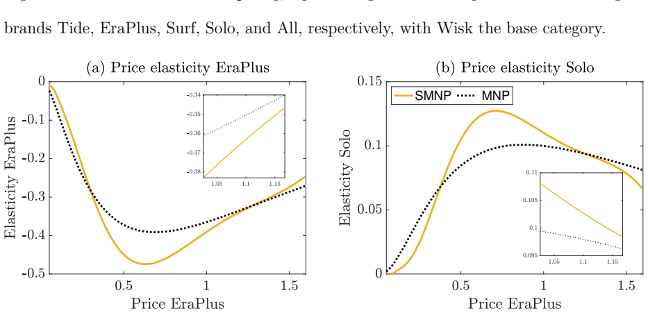
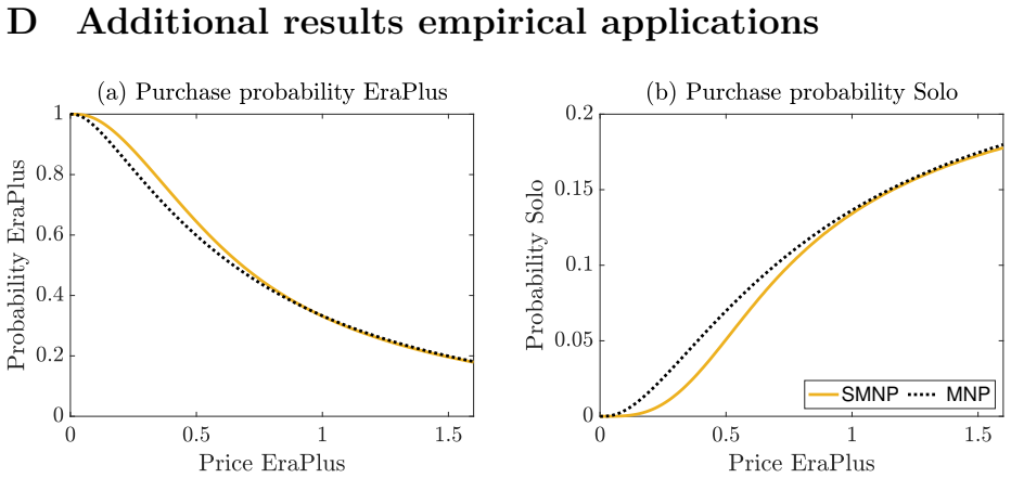
- In the paper's applications, allowing asymmetry changes own- and cross-price elasticities: the MNP understates price sensitivity for a focal detergent brand and misallocates substitution across ketchup brands.
- The sampler is practical for the datasets studied: all full conditionals except $\delta_1$ are closed-form Gibbs steps, with a single univariate Metropolis–Hastings update.
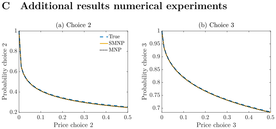
- When the data generating process is symmetric, SMNP shrinks toward MNP and does not lose predictive accuracy, so the added flexibility has little cost in symmetric settings.
- Because asymmetry is introduced through the latent utility distribution rather than observed gain/loss covariates, SMNP detects asymmetric responses without requiring reference prices or predictor transformations.
Reading between the lines
- If the identification concern is real, $\delta$ and alternative-specific intercepts are partially aliased, so posterior skewness should be checked for sensitivity to the intercept prior or to centering the skew-normal error at zero mean.
- The distributional asymmetry is silent about mechanism: loss aversion, brand loyalty, and switching costs can all produce similar shapes; letting $\delta$ depend on covariates would make mechanisms testable.
- The double augmentation strategy should carry over to skew-$t$ or related skew-elliptical errors because the conditionally Gaussian representation generalizes, adding tail robustness.
- A prior-predictive check for symmetry—comparing the observed difference in response to a price increase versus a price decrease with the range implied by the $\tau_\delta$ prior—would separate prior-induced from data-induced asymmetry.
Signed reviews
Editorial analysis
A structured set of objections, weighed in public.
Referee Report
Summary. The paper proposes a skewed multinomial probit (SMNP) model in which latent utilities follow a multivariate skew-normal distribution, allowing asymmetric choice responses. The authors introduce a reparameterization of the covariance matrix that enforces the MNP scale normalization and positive definiteness, a double data augmentation scheme yielding a Metropolis-Hastings within Gibbs sampler, and priors centered on a symmetric equicorrelated structure. Numerical experiments with symmetric and asymmetric DGPs and two empirical applications (laundry detergent and ketchup) are used to argue that SMNP recovers skewness, improves predictive accuracy, and changes implied price elasticities and substitution patterns.
Significance. The paper addresses a real gap in discrete choice modeling: the symmetry restriction of standard multinomial probit. If the identification and computational claims are correct, the SMNP model is a useful, parsimonious alternative to reference-price or random-coefficient approaches to asymmetry. The paper's numerical experiments are carefully designed with known DGPs and oracle comparisons, and the empirical evaluation uses repeated out-of-sample splits, which is a methodological strength. However, the identification proof is a necessary part of the contribution and is currently missing.
major comments (1)
- [Section 3.2, Eq. (7)] The claim that the reparameterization 'is key for identification' and that θ is 'the identified parameter vector' is not supported by a formal identifiability proof. The construction in Eq. (7) ensures only that every posterior draw satisfies the scale normalization Σ_11=1 and that Σ_u is positive definite; it does not establish that the map from θ to the multinomial choice probabilities is injective. Because the multivariate skew-normal error has nonzero mean √(2/π)δ, a change in δ can be compensated by an opposite change in the alternative-specific intercepts contained in X_i (Eq. 3) so that the conditional mean of Z_i is unchanged. The paper does not provide a rank condition or an argument showing that the higher-order cumulants of the skew-normal are separately identified from polychotomous choices. Without this, the MCMC sampler is operating on a parameter vector whose posterior may contain ridges, and the reported posterior densities for δ in Figures 2, 4, 5, and 7 cannot be interpreted as conclusive evidence of identification. This is load-bearing because the abstract and Section 6 list 'fully identified' as a main contribution.
minor comments (4)
- [Section 5.1] The sentence 'In addition, we also apply the Giacomini–White test directly to the' is incomplete and should be finished or removed.
- [Section 1] The word 'difficult' appears in the introduction and should be corrected to 'difficult'.
- [Appendix A, Eq. (21)] The expression for the expectation of ψ is written as V/((J+3)−(J−1)−1), which simplifies to V/3; the intermediate notation is confusing and could be simplified.
- [Table 2] In the ketchup panel, the CLS3 entries for MNP and SMNP are identical (−0.4778) but the MNP entry is flagged with a star; the note should explain the convention for ties.
Circularity Check
No significant circularity: out-of-sample predictions and fixed priors make the central claims independent of fitted inputs; the identification assertion is a rigor gap, not a circular reduction.
full rationale
The paper's derivation chain is self-contained against external benchmarks. The SMNP likelihood is built from the standard multivariate skew-normal stochastic representation in equation (5), and the reparameterization in equation (7) is derived in Appendix A as a Cholesky-based restriction that enforces the scale normalization Sigma_11 = 1 and positive definiteness; it is not fitted to outcome data. The numerical experiments generate data from known DGPs and compare predictive distributions to an oracle, with out-of-sample scoring reported in Table 1, and the empirical applications use repeated 80/20 train/test splits described in Section 5. The prior on the skewness vector delta is centered at zero and fixed before seeing outcomes, so the model does not fit skewness to the quantities later reported as predictions. No fitted parameter is renamed as a prediction, and no load-bearing step is justified solely by a self-citation. The self-citations to Loaiza-Maya and Nibbering (2022, 2023) concern dataset conventions and earlier MNP estimation methods, not the SMNP identification claim. The one notable weakness is that identification of theta = (beta, delta, gamma, psi) is asserted in Section 3.2 rather than proven: equation (7) guarantees that posterior draws satisfy the normalization and positive definiteness, but the paper does not supply a rank or injectivity condition showing that the map from theta to the multinomial choice probabilities is one-to-one. That is a mathematical rigor concern, not a circular step, because no equation in the paper reduces a predicted quantity to an input fitted value or derives the central claim from a self-referential definition. Therefore no circular step can be identified from the text.
Assumptions & free parameters
free parameters (3)
- tau_delta =
0.1936
- tau_gamma =
0.9 * UB_gamma (formula in Appendix A.2)
- c =
0.995
assumptions (5)
- standard math The stochastic representation of the multivariate skew-normal distribution in equation (5) holds for delta defined via alpha and Sigma.
- standard math The multivariate skew-normal family is closed under affine transformations, so that Z_i ~ SN_J(X_i beta, Sigma, alpha).
- domain assumption The model in (1)-(2) with J differenced utilities and threshold zero is observationally equivalent to a multinomial probit with J+1 alternatives and base utility fixed at zero.
- domain assumption The prior on (beta, delta, gamma, psi) is proper and yields a proper posterior, so that MCMC draws describe a well-defined posterior distribution.
- domain assumption The proposed sampler is geometrically ergodic and produces reliable posterior summaries in the reported runs.
Cite this review
Pith. "Pith review of A Multinomial Probit Model for Asymmetric Choice Responses." pith.science (2026). https://pith.science/paper/G272IU2E
@misc{pith2026260810336,
  author       = {Pith},
  title        = {Pith review of: A Multinomial Probit Model for Asymmetric Choice Responses},
  year         = {2026},
  howpublished = {\url{https://pith.science/paper/G272IU2E}},
  note         = {Machine review of arXiv:2608.10336}
}
read the original abstract
Standard multinomial probit (MNP) models specify symmetric latent utility distributions, implying that choice probabilities respond symmetrically to positive and negative covariate shifts of the same magnitude. This restriction is often implausible in empirical choice settings and can lead to misleading elasticity and substitution predictions. We propose a skewed multinomial probit (SMNP) model that captures asymmetric choice responses by specifying a multivariate skew-normal distribution for the latent utilities. The model preserves the flexible substitution patterns of the MNP framework, introduces alternative-specific skewness parameters, and nests the standard MNP model when skewness is zero. Introducing skewness creates identification and computational challenges because the skewness parameters interact with the MNP scale normalization and disrupt the conditional Gaussian updating structure used in Bayesian MNP estimation. We address these challenges through a covariance reparameterization that enforces identification and positive definiteness by construction, interpretable priors on the identified parameter space, and a double data-augmentation scheme that yields a Metropolis-Hastings within Gibbs sampler. Numerical experiments and applications to consumer choice data show that SMNP recovers asymmetric choice responses, improves probabilistic prediction, and produces economically meaningful differences in price elasticities and substitution patterns.
Figures


Figures from the paper (7 more)




Reference graph
Works this paper leans on
-
[1]
Let 𝐿21𝐿11 = 𝛾 , so that 𝐿21 = 𝛾 √1−𝛿2 1 . Since 𝐿22 is a lower-triangular matrix with real and positive diagonal entries, we have 𝐿22𝐿⊤ 22 = 𝜓 is a positive-definite matrix. Under this parameterization, Σ𝑢 can be expressed as Σ𝑢 = ⎡ ⎢ ⎣ 1 − 𝛿 2 1 𝛾⊤ 𝛾 𝜓 + 𝛾𝛾 ⊤ 1−𝛿2 1 ⎤ ⎥ ⎦ . (15) 31 This parameterization allows us to place priors directly on (𝛿, 𝛾, 𝜓). S...
work page 2004
-
[2]
= 1−𝕍(𝛿 1), which always follows by the fact that 𝔼(𝛿2
-
[3]
Second 𝔼(𝛾) = 0.5 × 1 𝐽−1 , which can be easily imposed by setting 𝐵𝛾 = 0.5 × 1𝐽−1
= 𝕍(𝛿 1). Second 𝔼(𝛾) = 0.5 × 1 𝐽−1 , which can be easily imposed by setting 𝐵𝛾 = 0.5 × 1𝐽−1 . Third, we must impose the condition 𝔼 [𝜓 + 𝛾𝛾 ⊤ 1 − 𝛿 2 1 ] = 0.5 × 1 𝐽−1 1⊤ 𝐽−1 + (0.5 − 𝜏𝛿)𝐼𝐽−1 , (20) where 𝜏𝛿 must be chosen such that the right-hand side of ( 20) is positive definite. It is straightforward to show that the smallest eigenvalue of this matri...
work page 2000
-
[4]
Otherwise, the draw is rejected and we retain the previous value, ̃𝛿(𝑟) 1 = ̃𝛿(𝑟−1) 1 . Here, the proposal density 𝑞( ̃𝛿1) is constructed via a Laplace approximation to the condi- tional posterior of ̃𝛿1. Specifically, we numerically maximize the log of posterior ( 30) to obtain the Maximum A Posteriori (MAP) estimate ̃𝛿1𝑀𝐴𝑃 , which corresponds to the mod...
work page 2010
Reviewed August 15, 2026 · model on record in the stance chip above.
Discussion (0). Continue with ORCID to comment.