REVIEW 2 major objections 5 minor 3 references
Recursive Adaptive Importance Sampling with Optimal Replenishment
T0 review · 2 major / 5 minor · reviewed 2026-08-04 · deepseek-v4-flash
Pith's one-line read Exponential replenishment keeps recursive importance sampling both fast and stable.
desk verdict The RAISOR algorithm is a sensible integration of recursive Bayesian updating with adaptive importance sampling, and the exponential-replenishment cost story is clean, but the theorem as written has a load-bearing mismatch between the definition of θ* and the BvM theorem it invokes — fix that and the paper is solid. read the letter →
The pith
A machine-rendered reading of the paper's core claim, the machinery that carries it, and where it could break.
The reading
What carries the argument
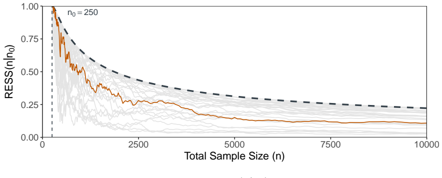
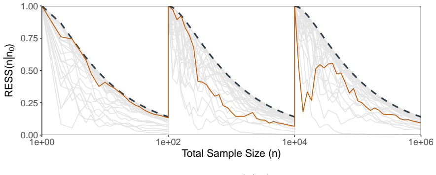
The relative effective sample size (RESS), defined as {1 + χ²-divergence([θ|y1:n] ∥ [θ|y1:n0])}^{-1}, is the object that tracks sample degeneracy. The argument shows that RESS(n|n0) can be rewritten as a ratio of integrals of a likelihood-ratio power against the partial posterior density, then uses the Bernstein-von Mises theorem under misspecification to replace the partial posterior by a normal density. This reduces the asymptotic problem to a product of Gaussian integrals, yielding the closed-form limiting RESS identity and the exponential-replenishment optimality conclusion.
What would settle it
Run the method on repeated i.i.d. datasets under the paper's regularity conditions, record the RESS at exponentially spaced replenishment times with a fixed α, and compare the empirical distribution to {α(2−α)}^{d/2} exp(−((1−α)/(2−α)) z' M_{θ*} z); a systematic mismatch for large n would refute the claimed convergence. Separately, under dependent observations generated by, say, a Gaussian process or an AR(1) model, check whether increasing the replenishment growth rate beyond exponential still maintains a non-degenerate RESS at O(n^p) cost; a collapse would confirm the paper's conjecture that
Extended reading notes
Core claim
The paper's central result is Theorem 3.1: under i.i.d. observations with mild regularity conditions, the relative effective sample size RESS(n|n0) of a sample that was replenished at time n0 converges in distribution to a closed-form random variable, RESS_{θ*,α}(z) = {α(2−α)}^{d/2} exp(−((1−α)/(2−α)) z' M_{θ*} z), where z is standard normal, α = lim n0/n, and M_{θ*} is a sandwich-type matrix built from the score and the prior-expected information at the limiting parameter θ*. This limit is non-degenerate for α in (0,1) and collapses to zero as α→0. Consequently, replenishment times that grow exponentially achieve an asymptotically optimal trade-off: per-Monte-Carlo-sample cost stays at O(n^
Load-bearing premise
The i.i.d. assumption on the observations is load-bearing: the proof of Theorem 3.1 breaks without independence, and the paper itself says the RESS behavior must then be assessed case by case, even though the method is applied to dependent spatial data.
Editorial extensions
If this is right
- If Theorem 3.1 is right, a practitioner can set replenishment times to grow exponentially and obtain a provable balance: O(n^p) cost per Monte Carlo sample with a non-degenerate RESS, matching the asymptotic cost of Metropolis-Hastings while remaining parallel-friendly.
- The limiting distribution gives a quantitative way to choose replenishment thresholds: the deterministic factor {α(2−α)}^{d/2} yields the bound n ≤ c(r_min, d) n0 for guaranteed quality loss, which the paper turns into concrete heuristics for batch sizes and thresholds.
- Because the theorem holds under model misspecification, the method is advertised as robust to wrong models, with the sandwich matrix M_{θ*} governing the speed of sample degeneration.
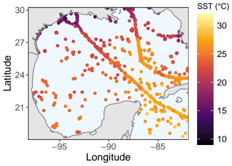
- In the Gaussian-process regression and sea-surface-temperature experiments, RAISOR achieves a substantially higher effective-sample-size-per-minute than the MCMC baseline, suggesting the theoretical cost-quality trade-off translates into practical speedups.
- The recursive weight update can be batched, so communication between parallel processors is reduced, making the method more efficient in distributed computing environments.
Reading between the lines
- The paper's stochastic-threshold replenishment rule (trigger on estimated RESS falling below r) is its practical default, yet the optimality theorem is proven only for deterministic exponential schedules; a natural extension is to prove that the threshold rule inherits an exponentially growing sequence of replenishment times in an appropriate asymptotic regime.
- The RESS trajectory itself could be repurposed as a model-checking diagnostic: the paper shows that misspecification with W_{θ*} > V_{θ*} accelerates sample degeneracy, so a fitting run that repeatedly hits low RESS values may flag overconfident posteriors, not merely bad sampler settings.
- The method's reliance on mixture-of-normals approximations of the partial posterior suggests it could extend to online learning and multimodal targets through annealed bridging, but its effectiveness in high dimensions is expected to degrade, since the dimension d enters exponentially in the deterministic RESS bound.
- A concrete testable extension: in correlated or non-i.i.d. data (where Theorem 3.1 does not apply), the paper conjectures the RESS limit must be assessed case by case; simulations with Matérn spatial dependence could reveal whether exponential replenishment still keeps a bounded, healthy RESS empirically.
Editorial analysis
A structured set of objections, weighed in public.
Referee Report
Summary. The paper proposes RAISOR, a recursive adaptive importance sampling algorithm that alternates fast recursive weight updates with occasional sample replenishment. The central theoretical contribution is Theorem 3.1, which states that, under i.i.d. observations and possible model misspecification, the relative effective sample size RESS(n|n0) with n0 = alpha_n n and alpha_n -> alpha has the non-degenerate limiting distribution RESS_{theta*,alpha}(z) = {alpha(2-alpha)}^{d/2} exp(-((1-alpha)/(2-alpha)) z' M_{theta*} z). This result is used to argue that exponentially growing replenishment times achieve an asymptotically optimal trade-off between O(n^p) Monte Carlo cost and sample quality. The paper also provides detailed implementation guidance, two simulated experiments (conjugate normal and Gaussian process regression with Vecchia approximation), and an application to sea surface temperature data in the Gulf of Mexico. The proof in Appendix A is substantial and explicitly builds on Kleijn & Van der Vaart (2012).
Significance. If Theorem 3.1 is made correct, the paper makes a useful contribution: it gives a concrete asymptotic characterization of degeneracy in a recursive importance sampling scheme, explains why exponential replenishment is the right growth rate, and provides practical heuristics with extensive appendices. The explicit limiting formula, including the dependence on alpha and on the asymptotic covariance structure, is a valuable diagnostic. The paper also carefully states the limitations of the i.i.d. assumption and applies the method to a challenging NNGP spatial model. The main problem is that two definitions in the theorem statement are inconsistent with the proof: the objective defining theta* is not the KL objective required by the cited Bernstein-von-Mises theorem, and W_{theta*} is defined as a vector while used as a matrix. These are fixable locally, but as submitted the theorem cannot be verified.
major comments (2)
- [Section 3.1, Eq. (14); Appendix A, Eq. (55)] Eq. (14) defines theta* = argmin E*([y1]*/[y1|theta]), an expected density-ratio (chi-squared type) objective, but the proof relies on Kleijn & Van der Vaart (2012), whose Bernstein-von-Mises theorem requires theta* to be the KL minimizer, i.e., the maximizer of E* log[y1|theta]. The first-order condition for Eq. (14) is E*[(f*/f_{theta*}) ldot(theta*)] = 0, not E*[ldot(theta*)] = 0. Consequently, the score central limit theorem used in Lemma A.2, Eq. (55), is generally false: sqrt(n-n0) times the average score has mean sqrt(n-n0) E*[ldot(theta*)], which diverges unless E*[ldot(theta*)] = 0. Since the limiting RESS derivation rests on this CLT, the theorem as stated is not justified. Please change Eq. (14) to the KL-minimizing definition (or supply a separate proof for the density-ratio objective).
- [Theorem 3.1, Eq. (18); Appendix A, Lemma A.2] W_{theta*} is defined as E*(d/dtheta log[y|theta] | theta=theta*), which is a d-dimensional vector, but it is subsequently used as a positive-definite d x d covariance matrix: the theorem writes W_{theta*}^{1/2}, and Lemma A.2 uses W_{theta*} in normal limits such as Eq. (55) and Eq. (56). The definition should be W_{theta*} = E*[ldot(theta*) ldot(theta*)'], the expected outer product of the score vector. As written, M_{theta*} = (W^{1/2})' V^{-1} (W^{1/2}) is ill-defined and the proof's algebra cannot be checked.
minor comments (5)
- [Section 2.3.2] In the cost discussion, the text says 'the cost per Monte Carlo sample C_W of recalculating the weights throughout the procedure will be C_R(n) = O(sum_{k=1}^n k^p)'. The symbol C_R is used instead of C_W. Please fix the notation.
- [Section 4.1.1] The posterior mean formula for the conjugate normal model is written as mu_n = sigma_n^2 {sigma_0^{-2} mu_0}, omitting the data term n sigma^{-2} ybar. If the simulations silently use ybar = 0, please state that; otherwise the formula is incorrect.
- [Eq. (11)] The estimator in Eq. (11) is typeset as '\RESS' with a literal backslash. It should be '\widehat{RESS}' or a similar estimator notation.
- [Section 2.3.3 and Theorem 3.1] The notation for replenishment times, n*_k = ceil(alpha^{-k} n) or ceil(alpha_n^{-k}), is ambiguous in the typeset equation. Please clarify whether the multiplier 'n' is part of the argument or a subscript.
- [Appendix C, Example C.2] The definition of z in Example C.2 is garbled: 'z = { n/((n-n0)n0)}^{-1/2} W^{-1/2} V(...)' should be rewritten so that the scaling and the random variable are unambiguous.
Circularity Check
No load-bearing circularity; Theorem 3.1 is a genuine asymptotic derivation from external misspecified-BvM results and a CLT.
full rationale
The central theoretical claim, Theorem 3.1, is not circular. RESS is defined in Eq. (7) as a decreasing function of the chi-squared divergence between two posteriors; this definition is independent of the theorem's conclusion. The limiting distribution in (17) is obtained in Appendix A by (i) replacing the initial posterior by a normal approximation via Kleijn & Van der Vaart's misspecified Bernstein-von-Mises theorem (an external, parameter-free result), and (ii) analyzing the likelihood-ratio integral with a CLT for the score; this is a proof from stated assumptions, not a restatement of the input. The 'optimal replenishment' claim follows from the theorem plus the explicit O(n^p) cost bounds in (9)-(10), so it is a consequence rather than an encoding of the answer. The only self-citations are to Hooten et al. (2021) and Ren et al. (2025); these are used as background and as the naming source for 'importance PP-RB', and neither carries the proof of Theorem 3.1, so they are not load-bearing. The paper's own Section 5 limitation that independence is crucial and that dependent cases must be assessed case-by-case is an honest caveat, not an admission of circularity. One correctness concern should be noted separately: Eq. (14) defines theta* as the minimizer of E*([y1]*/[y1|theta]), whereas the misspecified BvM theorem used in Lemma A.2 concerns the KL minimizer (maximizer of E* log[y|theta]); as written, the centered score in (55) has no stated zero-mean property, so the CLT step lacks justification. This is a potential gap in the proof's rigor, but it is not a circular reduction of the theorem to its own conclusion, so it does not raise the circularity score.
Assumptions & free parameters
free parameters (7)
- alpha (replenishment growth factor) =
2/3 in applications
- r_min (minimum RESS threshold) =
0.1
- r (replenishment threshold) =
0.2
- M (number of Monte Carlo samples) =
50000
- number of mixture components =
10
- initial sample size n0 =
10
- B (in-between batch sizes) =
20
assumptions (6)
- domain assumption Observations are i.i.d. under the true distribution and the model.
- domain assumption There exists a unique theta* in the interior of Theta minimizing E*([y1]*/[y1|theta]).
- standard math The log-likelihood is differentiable at theta* with a Lipschitz condition and a quadratic expansion of the local log-likelihood ratio.
- domain assumption The MLE exists and is consistent for all n > n0.
- standard math The prior density is continuous and positive in a neighborhood of theta*.
- standard math The Bernstein-von Mises theorem under misspecification (Kleijn & Van der Vaart 2012).
Cite this review
Pith. "Pith review of Recursive Adaptive Importance Sampling with Optimal Replenishment." pith.science (2026). https://pith.science/paper/GERI4YRX
@misc{pith2026250908102,
  author       = {Pith},
  title        = {Pith review of: Recursive Adaptive Importance Sampling with Optimal Replenishment},
  year         = {2026},
  howpublished = {\url{https://pith.science/paper/GERI4YRX}},
  note         = {Machine review of arXiv:2509.08102}
}
read the original abstract
Increased access to computing resources has led to the development of algorithms that can run efficiently on multi-core processing units or in distributed computing environments. In the context of Bayesian inference, many parallel computing approaches to fit statistical models have been proposed in the context of Markov Chain Monte Carlo methods, but they either have limited gains due to high latency cost or rely on model-specific decompositions. Alternatively, adaptive importance sampling, sequential Monte Carlo, and recursive Bayesian methods provide a parallel-friendly and asymptotically exact framework with well-developed theory for error estimation. We propose a recursive adaptive importance sampling approach that alternates between fast recursive weight updates and sample replenishment steps to balance computational efficiency while ensuring sample quality. We derive theoretical results to determine the optimal allocation of replenishing steps, and demonstrate the efficacy of our method in simulated experiments and an application of sea surface temperature prediction in the Gulf of Mexico using Gaussian processes.
Figures

Figures from the paper (3 more)


Reference graph
Works this paper leans on
-
[1]
(sampling) one can efficiently generateθ1,...,θ M iid ∼[θ|η]for any choice ofη
-
[2]
(tractability)[θ|η]is analytically available up to a proportionally constant and cheap to evaluate
-
[3]
(closeness) for allε>0, there isηsuch thatD χ2([θ|y1:n]∥[θ|η])<ε. The sampling condition ensures fast replenishment, tractability makes it possible to calculate exact IS weights (assuming[θ|y1:n]is also tractable), and closeness guarantees that one can always increaseRESS(n|n0)after replenishment for some choice ofη. Takingθ to be continuous, the first tw...
work page 1995
Reviewed August 4, 2026 · model on record in the stance chip above.
Discussion (0). Continue with ORCID to comment.