REVIEW 3 major objections 3 minor 16 references
Properties of the Center of Gravity as an Algorithm for Position Measurements
T0 review · 3 major / 3 minor · reviewed 2026-08-14 · deepseek-v4-flash
Pith's one-line read Centroiding error is one Fourier series—and crosstalk can kill it
desk verdict A correct and useful derivation of the COG discretization error, with one real definitional gap in the 'ideal detector' section that should be fixed before this is relied upon. read the letter →
The pith
A machine-rendered reading of the paper's core claim, the machinery that carries it, and where it could break.
The reading
What carries the argument
The load-bearing object is the sampled signal train $s_\varepsilon(x)=f(x-\varepsilon)\sum_n\delta(x-n\tau)$, whose Fourier transform is evaluated by the Poisson identity $S_\varepsilon(\omega)=\tau^{-1}\sum_k F_\varepsilon(\omega-2\pi k/\tau)$. Because the integrating detector converts the signal to $f(x-\varepsilon)$ through a convolution with a rectangular window, $F_\varepsilon(\omega)=[2\sin(\omega\tau/2)/\omega]\Phi(\omega)e^{-i\varepsilon\omega}$, and the COG formula $x_g=i S_\varepsilon'(0)/S_\varepsilon(0)$ turns the derivative into the sine series of Eq. (6). The same machinery is reused in two further forms: the dual Shannon/WKS series expresses $\Phi$ through the form factors $\Phi(2\pi n/D)$, and a contour-residue summation converts the resulting double series into the practical expression Eq. (13). For crosstalk, the response function $p$ enters through its Fourier transform $P$ and its derivative, and the condition for an ideal detector is stated directly as a vanishing weighted sum of shifted response copies.
What would settle it
Scan a known, sharp source across one pitch of a strip or pixel detector, measure both the mean signal shape and the centroid $x_g(\varepsilon)$, and compare the residual $x_g-\varepsilon$ with the series in Eq. (6) using the independently measured Fourier transform $\Phi$. Agreement within noise supports the model; systematic position-dependent deviations that do not follow the predicted coefficients would falsify it. A separate direct test: a detector with triangular crosstalk of range $2\tau$ should show $x_g=\varepsilon$ to within noise for every signal distribution; any periodic wiggle in the residual rules out the ideal-detector claim.
Extended reading notes
Core claim
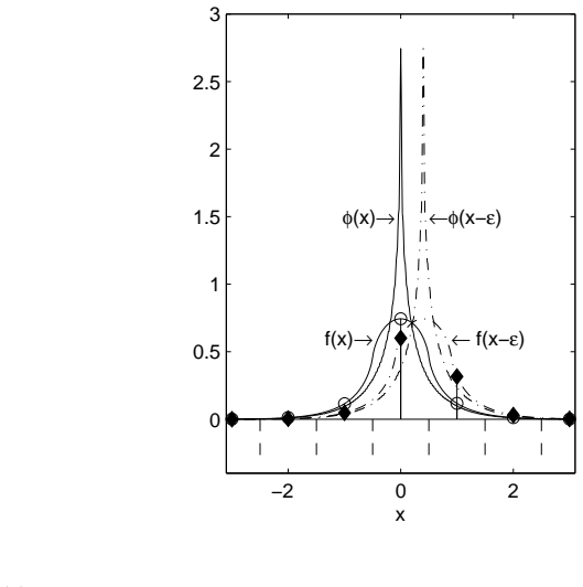
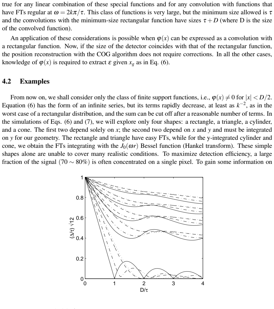
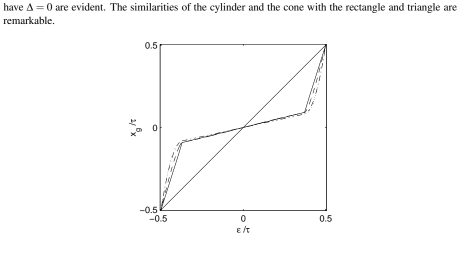
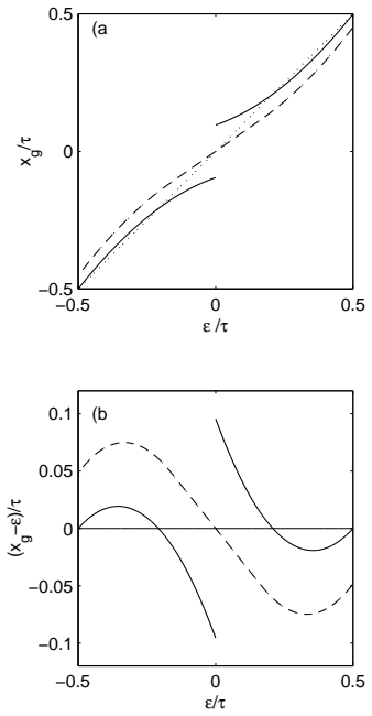
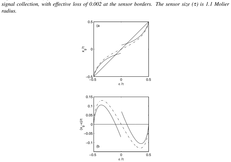
On the paper's own terms, the central result is Eq. (6): for an infinite periodic array of ideal integrating sensors with pitch $\tau$, the COG estimate is $x_g = \varepsilon + (\tau/\pi)\sum_{k\ge1}(-1)^k k^{-1}\sin(2\pi k\varepsilon/\tau)\Phi(2\pi k/\tau)$, where $\varepsilon$ is the true impact position and $\Phi$ is the Fourier transform of the mean signal distribution. The discretization error is therefore not a statistical nuisance but a deterministic function of the signal spectrum at the sampling frequencies. The paper further proves that the error vanishes when $\Phi(2\pi k/\tau)=0$ for all $k>0$, a condition broader than the Whittaker-Kotelnikov-Shannon band limit, and exhibits finite-support shapes such as rectangular signals with integer-multiple widths and triangular signals with even-multiple widths that satisfy it. It then extends the analysis to crosstalk: if the detector response $p(x,\tau_1)$ satisfies $\sum_n (x-n\tau)p(x-n\tau,\tau_1)=0$, in particular triangular crosstalk of range $2\tau$, the COG equals $\varepsilon$ for any signal distribution. Finite clusters of sensors are treated too, and they produce discontinuities in $x_g(\varepsilon)$ at the points where the set of sensors changes.
Load-bearing premise
The whole Fourier-series correction rests on treating the detector as an infinite periodic row of identical sensors whose collected signal is exactly a shift-invariant convolution of the mean signal with a fixed response function; real detectors with finite size, varying strip widths or gains, calibration errors, or unread gaps only approximate this model.
Editorial extensions
If this is right
- For any detector that matches the infinite periodic model, the systematic position error can be removed by inverting Eq. (6) or using Eq. (13), without per-detector Monte Carlo tuning.
- A detector engineered to have triangular crosstalk of range $2\tau$, or any response satisfying $\sum_n (x-n\tau)p(x-n\tau,\tau_1)=0$, would be unbiased for every signal distribution.
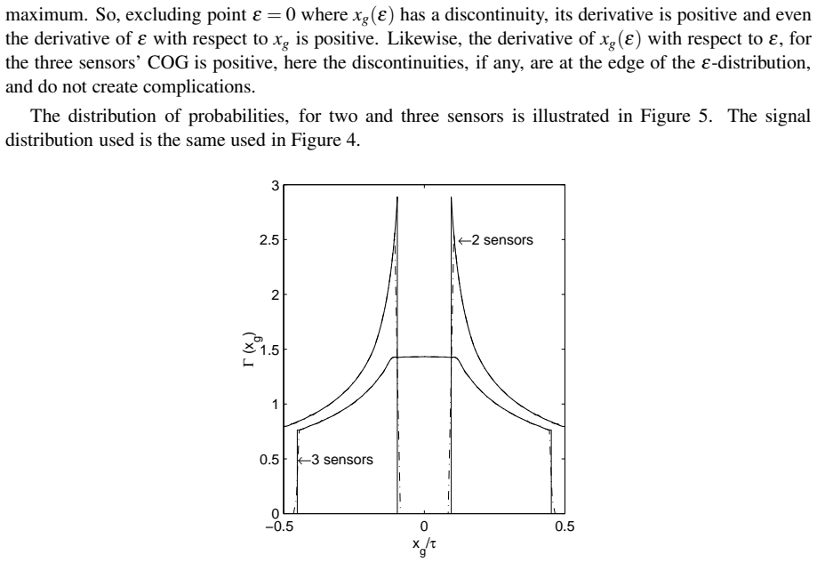
- Cluster-size cuts create discontinuities in $x_g(\varepsilon)$ at sensor boundaries; subtracting a fixed bias mixes incompatible two-sensor and three-sensor algorithms and cannot be fixed by a smooth polynomial correction.
- Given a large sample of equivalent hits with a uniform distribution of true positions, the histogram of $x_g$ yields $\varepsilon(x_g)$ by Eq. (25), and when the signal support fits within one pitch it also reconstructs the signal shape.
- The explicit formulas for crosstalk, noise, inter-strip calibration errors, cracks, and off-axis crystals make the same equations a compact simulation tool for real strip and crystal calorimeters.
Reading between the lines
- The ideal-detector condition suggests a concrete design target for silicon strip and pixel detectors: tune inter-strip capacitive coupling toward a triangular profile with range exactly twice the pitch, so centroids need no correction at all; this is an engineering consequence the paper states mathematically but does not develop as a fabrication recipe.
- Because only the values $\Phi(2\pi k/\tau)$ enter the correction, the scheme should transfer directly to imaging and star-tracker centroiding wherever the point-spread function is known, not just to particle detectors.
- The predicted infinite peak in the $x_g$ probability density when the signal support $D\le\tau$ is a testable signature: a histogram of centroids from a source narrower than one pixel should show a sharp spike near zero, distinguishing this model from generic smoothing.
- The boundary-discontinuity analysis implies that any empirical bias curve subtracted from cluster centroids is only valid for a fixed sensor count; switching cluster sizes in the same analysis introduces uncorrectable systematic jumps.
Signed reviews
Editorial analysis
A structured set of objections, weighed in public.
Referee Report
Summary. The paper analyzes the center-of-gravity (COG) algorithm for one-dimensional position measurements in periodic detector arrays. The central result of Section 3.3 is an explicit formula, Eq. (6), for the systematic discretization error of the COG as a Fourier series whose coefficients are values of the Fourier transform of the average signal distribution at multiples of the sampling frequency. The paper then studies conditions under which this error vanishes, derives a resummed form of the series for finite-support signals in Section 5.3, generalizes the analysis to crosstalk and non-perfect spatial integrators in Section 6, treats finite sensor sets, noise, and fluctuations, and concludes with a claimed construction of an 'ideal detector' whose crosstalk eliminates the discretization error for any signal distribution.
Significance. If the results hold, the paper provides a useful analytical framework for correcting COG systematic errors in position-sensitive detectors, with direct applications to calorimeters and silicon strip trackers. The derivation of Eq. (6) is clean and is benchmarked against known special cases, including the Euler sine series in the delta-function limit and the Lau-Pyrlik conjecture. The paper also gives explicit simulation formulas. However, the 'ideal detector' claim, which is one of the advertised headline results, is under-specified as stated: the vanishing-moment condition alone is insufficient, and the paper's own derivation in Section 6.6 relies on an additional uniformity condition that is not included in the abstract or in the standalone definition. This is fixable, but it must be corrected before the central claim is accepted as stated.
major comments (3)
- [Section 6.6 and abstract] The definition of an ideal detector as a crosstalk function satisfying sum_n (x - n tau) p(x - n tau, tau_1) = 0 is insufficient for the claimed conclusion x_g(epsilon) = epsilon for any signal distribution. The derivation on the page with Eq. (14) explicitly uses the uniformity condition sum_n p(x - n tau, tau_1) = 1 to cancel the term involving x' after interchanging the sum and integral. Without uniformity, the zero-first-moment condition does not imply x_g = epsilon: for symmetric p supported on [-tau, tau] of the form p(x) = (tau - x) r(x) on [0, tau] with r symmetric about tau/2 but not constant, one has sum_n (x - n tau) p(x - n tau) = 0 identically, but M_0(x) = sum_n p(x - n tau) = tau r(x) is not constant, and the resulting COG is a weighted average of y M_0(y) rather than epsilon. The uniformity condition should be added to the definition of ideal detector and to the abstract.
- [Section 5.3, Eq. (13)] The summation leading to Eq. (13) is compressed, and the sawtooth function is defined inconsistently: the text states Theta(xi) = xi - floor(xi + 1/2), while Eq. (13) states Theta(xi) = xi - floor(xi - 1/2). These differ on half-integers and affect numerical implementation. The authors should specify the exact convention used in Eq. (13) and, if both forms are acceptable up to integer shifts, state that explicitly and verify that the residues are unchanged.
- [Section 6.6] The reference to 'Eq. (24)' in the ideal-detector derivation is incorrect: Eq. (24) is the probability-density transformation formula, not the expression for x_g(epsilon). The derivation uses the expression for x_g following from Eq. (14), so the equation numbering should be corrected and the derivation should be made self-contained.
minor comments (3)
- [Section 5.1] The condition 'phi(x) = 0 for |x| <= D/2' should read 'phi(x) = 0 for |x| > D/2', or equivalently 'phi(x) != 0 for |x| < D/2', to match the intended finite-support statement.
- [Introduction] The section numbering in the introductory text does not match the actual structure of the paper; for example, the text refers to 'Section 2' and 'Section 3' in ways that do not correspond to the displayed section headings.
- [Section 7.2] The phrase 'the average distribution omega (x)' appears to be a typo for phi(x), and 'Molier radius' should be 'Moliere radius' throughout the figure captions and text.
Circularity Check
No significant circularity: Eq. (6) is derived from standard Fourier/Poisson identities and benchmarked against independent results; self-citations are motivational only.
full rationale
Eq. (6) is derived in Section 3.3 by differentiating Sε(ω) in Eq. (3), applying the Poisson identity Eq. (4), and using the explicit Fourier transform Fε(ω) = [2 sin(ωτ/2)/ω] Φ(ω) e^{-iεω}; no parameter is fitted, and the error series is determined by the Fourier transform Φ exactly as claimed. The checks against the Euler sine series and the Lau-Pyrlik conjecture use independent external results, and the η-function discontinuity [16] is a comparison, not an input. The 2019 preface cites several of the author's own later papers (arXiv:1606.03051, arXiv:1808.06708, INSTRUMENTS 2018 2 22, arXiv:1404.1968) but only for motivation, applications, and context; those citations do not supply any assumption used to derive Eq. (6) or the crosstalk theorems. The only notable defect is the 2019-added ideal-detector definition, which states only Σ_n (x−nτ)p(x−nτ,τ1)=0 while the proof in Section 6.6 uses both uniformity (Σ_n p(x−nτ,τ1)=1) and the vanishing first lattice moment; this is an under-specified definition or overclaim, not a circular reduction. Hence no circularity score above the minor self-citation level is warranted.
Assumptions & free parameters
assumptions (5)
- domain assumption The average signal distribution is shift invariant: for impact point epsilon it is exactly phi(x - epsilon), with phi real, symmetric, normalized and having a continuous, derivable Fourier transform.
- domain assumption The detector is an infinite regular array of identical ideal integrators of width tau, with no gaps or position-dependent losses.
- standard math Poisson summation formula and the WKS sampling theorem.
- domain assumption Crosstalk is a linear, shift-invariant convolution p(x - x', tau1) of finite range.
- domain assumption For the monotonicity proof in Section 6.5, phi and f are positive, continuous, derivable, single-maximum functions with D > tau.
Cite this review
Pith. "Pith review of Properties of the Center of Gravity as an Algorithm for Position Measurements." pith.science (2026). https://pith.science/paper/GK2BBGDF
@misc{pith2026190804447,
  author       = {Pith},
  title        = {Pith review of: Properties of the Center of Gravity as an Algorithm for Position Measurements},
  year         = {2026},
  howpublished = {\url{https://pith.science/paper/GK2BBGDF}},
  note         = {Machine review of arXiv:1908.04447}
}
abstract
The center of gravity $x_{g}= \sum_{i}E_{i} x_{i}/\sum_{i} E_{i}$ as an algorithm for position measurements is carefully analyzed. Many mathematical consequences of discretization are extracted. The origin of the systematic error of the algorithm is shown to be connected to the absence of band limits in the Fourier Transform of the signal distributions, which, owing to the intrinsic properties of the measuring devices, must have a finite supports. However, special signal distributions exist among the finite support functions which are free from the discretized error. In the presence of crosstalk, it is proved that some crosstalk spreads are able to eliminate the discretization error for any shape ({\em ideal detector}). For all other cases, analytical expressions and prescriptions are given to correct the error and to efficiently simulate various experimental situations.
Figures
Figures from the paper (5 more)
Reference graph
Works this paper leans on
-
[1]
A TLAS Collaboration.CERN-LHCC-94-43
- [2]
- [3]
-
[4]
CMS Collaboration, The Electromagnetic Calorimeter, C ERN/LHCC 1997-33
work page 1997
-
[5]
Wigmans, Calorimetry (Clarendon Press, Oxford, 2000 )
R. Wigmans, Calorimetry (Clarendon Press, Oxford, 2000 )
work page 2000
-
[6]
CMS Collaboration, Tracker Design Report, CERN/LHCC 19 98-6
- [7]
-
[8]
Bracewell, The Fourier Transform and Its Applicati on (McGraw-Hill, New Y ork, NY , 1986)
R.N. Bracewell, The Fourier Transform and Its Applicati on (McGraw-Hill, New Y ork, NY , 1986)
work page 1986
Show all 16 references
-
[9]
Champeney, A Handbook of Fourier Theorems (Cambrid ge University Press, Cambridge, UK, 1987)
D.C. Champeney, A Handbook of Fourier Theorems (Cambrid ge University Press, Cambridge, UK, 1987)
1987
-
[10]
Lau and J
K. Lau and J. Pyrlik, Nucl. Instrum. Methods A 366, 298 (1 995)
-
[11]
A. J. Jerri Proceedings IEEE 65, 1565 (1977)
1977
-
[12]
Lednev, Nucl
A.A. Lednev, Nucl. Instrum. Methods A 366, 292 (1995)
1995
-
[13]
Suhling, R
K. Suhling, R. W. Airey, B.L. Morgan, Nucl. Instrum. Met hods A 437, 393 (1999)
1999
-
[14]
Henrici, Applied Computational Complex Analysis (J ohn Wiley, New Y ork, NY , 1974)
P . Henrici, Applied Computational Complex Analysis (J ohn Wiley, New Y ork, NY , 1974). 27
1974
-
[15]
Alpat et al., Nucl
B. Alpat et al., Nucl. Instrum. Methods A 439, 53 (2000)
2000
-
[16]
Belau et al., Nucl
E. Belau et al., Nucl. Instrum. and Methods 214, 253 (198 3). 28
Reviewed August 14, 2026 · model on record in the stance chip above.
Discussion (0). Continue with ORCID to comment.