REVIEW 4 major objections 4 minor 43 references
Yau-YauAL: A computer tool for solving nonlinear filtering problems
T0 review · 4 major / 4 minor · reviewed 2026-08-07 · deepseek-v4-flash
Pith's one-line read YauYauAL packages the Yau-Yau nonlinear filter into open-source R software.
desk verdict A real R package for the Yau-Yau filter, but the paper's accuracy claims outrun its evidence and the demo builds the grid from the true state. read the letter →
The pith
A machine-rendered reading of the paper's core claim, the machinery that carries it, and where it could break.
The reading
What carries the argument
The load-bearing mechanism is the Yau-Yau algorithm's reduction of the nonlinear filtering problem to the Kolmogorov forward equation, combined with a finite-difference spatial discretization and a discrete sine transform (DST) solver. Given a drift f and observation h, the package builds a spatial grid, assembles derivative, transition, and observation matrices, then advances the conditional density forward in time and normalizes against the incoming observations. The paper cites the Yau-Yau convergence guarantee that the estimate converges to the true solution when the growth rate of the observation function |h| exceeds that of the drift |f|.
What would settle it
Run YauYauAL on a scalar linear-Gaussian model where the Kalman filter gives the exact posterior, using a simulation that does not reach the distribution's tails, and compare the package's estimated conditional mean and density with the exact values; divergence beyond the discretization error would show the grid-coverage assumption is load-bearing. A second check: run the cubic sensor problem with h(x)=x instead of h(x)=$x^{3}$, where the observation-growth condition is weaker, and see whether the estimates degrade.
Extended reading notes
Core claim
The central claim is that YauYauAL makes the Yau-Yau nonlinear filter practically usable as software. In the paper's account, the filter estimates a stochastic system's state from noisy observations by solving the Kolmogorov forward equation for the conditional density, and YauYauAL does this numerically with a finite-difference scheme and a discrete sine transform, taking only the drift f, the observation function h, and grid and time-step settings as inputs. The package is written in R with C++ kernels and includes a Shiny-based interactive interface for control and visualization. Its two numerical demonstrations show the Yau-Yau filter estimating states for the almost linear sensor problem and a three-dimensional cubic sensor problem.
Load-bearing premise
The numerical grid is constructed from the range of one simulated state path, so the result assumes that this path covers every region of state space where the true conditional density has meaningful mass; if the true state wanders outside that range, the finite-difference solution is not reliable.
Editorial extensions
If this is right
- Users who can write down f and h can run a nonlinear filter on their own system without implementing the mathematics or writing numerical solvers.
- The interactive interface lets parameters be adjusted and results inspected live, which makes the package usable for quick prototyping and teaching.
- The two demonstrations show the method tracking a scalar almost linear sensor and a three-dimensional cubic sensor, so the package is positioned as working beyond scalar textbook examples.
- Because the code is open-source and modular, researchers can replace or extend the numerical components for their own applications.
Reading between the lines
- The spatial grid is built from the range of one simulated trajectory (s <- seq(min(x), max(x)+Ds, by=Ds)), so the package's accuracy silently depends on that trajectory covering the density's support; a short or atypical simulation could produce estimates that are right only inside a truncated domain.
- The paper's convergence guarantee (observation growth exceeding drift growth) is not checked in the demonstrations; f=0 and f=cos(x) with h=x^3 both satisfy it, so a stress test with slower-growing observations would probe whether the software is trustworthy outside that regime.
- A natural validation the paper does not report is a comparison against the exact Kalman posterior in a linear-Gaussian case or against a particle filter in a nonlinear case; the finite-difference density could be checked for normalization and tail mass.
Editorial analysis
A structured set of objections, weighed in public.
Referee Report
Summary. The manuscript describes YauYauAL, an open-source R package with a C++ backend and a Shiny interface that implements the Yau-Yau nonlinear filter. The filter is realized by numerically solving the Kolmogorov forward equation via finite differences and a discrete sine transform. The paper provides installation instructions, a step-by-step usage guide with R code, two numerical examples (the almost linear sensor problem and the 3-D cubic sensor problem), and a short discussion. The central claims are that the package is stable, accurate, accessible to non-specialists, and suitable for a wide range of nonlinear filtering applications.
Significance. If the numerical implementation is reliable, YauYauAL would be a useful contribution: it packages a theoretically well-motivated filtering algorithm into a reproducible, open-source R tool with a graphical interface. The paper's strengths include public code on GitHub, a reproducible seed-based simulation workflow, the use of Rcpp for efficiency, and a modular design that invites extension. However, the current numerical evidence is too thin to support the accuracy and stability claims: the experiments are side-by-side visualizations only, and the computational domain is chosen from the true simulated state path, which is both impractical for real applications and unexamined with respect to boundary effects. The paper therefore needs additional validation and methodological guidance before its central claims can be accepted.
major comments (4)
- [§3.3, code lines 2–4] The computational grid is constructed from the true simulated state trajectory: `s <- seq(min(x), max(x)+Ds, by=Ds)`, where `x` is the output of `Simulate_State_Obser` in §3.2. This is load-bearing for the paper's claim of a stable and accurate filter. First, in any real filtering problem the true state is unobserved, so the documented workflow cannot be applied to actual data, and the paper gives no instruction for choosing the grid from the observations `y` or from prior state bounds. Second, the discrete sine transform solver referenced in §3.4 imposes zero Dirichlet boundary conditions, so if the conditional density has nontrivial mass outside `[min(x), max(x)+Ds]`, the numerical solution is corrupted. The paper reports no grid-refinement study, no domain-size sensitivity analysis, and no check that the density mass lies inside the domain. Section 5 acknowledges that performance may depend on the system, but it does not connect this to domain choice. I recommend adding explicit guidance for grid selection from observables or prior bounds, and a sensitivity/refinement experiment that demonstrates domain adequacy.
- [§4.1, Eq. (2) and Figure 4] The experimental setup is internally inconsistent. Equation (2) states a scalar model with x(t), y(t) in R, but the parameter list immediately says Dim = 3, and Figure 4 displays only "Dimension 1". The same ambiguity occurs in §4.2: Equation (3) is scalar, yet the text refers to a "3-D Cubic sensor" and Figure 5 shows three dimensions. The paper does not explain whether the three dimensions are independent scalar sensors, a vector-valued generalization of the stated model, or something else. Because the numerical experiments are the only evidence for the algorithm's performance, this ambiguity prevents the reader from reproducing the results or assessing whether the stated model is actually the one being solved.
- [§4, Figures 4 and 5] The numerical evaluation consists solely of side-by-side plots of the true state and the filter estimate, with no error metrics, no convergence checks, and no comparison to standard baselines such as the particle filter or the extended Kalman filter. The abstract's claim that the method "ensures a stable and accurate solution" is therefore not substantiated. The paper should report at least one quantitative accuracy measure (e.g., root mean square error over time) and a comparison to a reference filter, plus a grid-refinement or domain-dependence check, before making this claim.
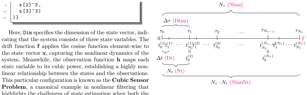
- [§3.1, code block] The example setup is not reproducible as written because of an internal inconsistency in the parameter definitions. The code sets `T <- 5`, but the surrounding text states "the terminal time T is set to 20," and the comments give `Ntau <- as.integer(T/Dtau) # 4000` and `NtNtau <- as.integer(T/Dt) # 20000`, which are only consistent with T = 20. The later call in §3.2 uses Ntau = 4000 and NtNtau = 20000, again matching T = 20. The manuscript should correct the code or the text so that the demonstration can actually be run.
minor comments (4)
- [Abstract and §1] There are several typographical and spacing errors, including "ccurate estimation" in the introduction and the run-together text "estimationorforecastsarecomputediterativelyandinreal-time." These should be corrected.
- [§3.4] The sentence "The Discrete Sine Transform to efficiently solve the Kolmogorov equation for accurate state estimation in nonlinear systems" is missing a verb and should be rephrased.
- [§3.5] The claim of "real-time parameter adjustment" in the abstract is qualified by the statement that Shiny "might not update the results in real-time" for custom filters; the paper should reconcile these statements or clarify what "real-time" means in this context.
- [§5] The Discussion is generic and does not mention the true-state dependence of the grid construction or the need for boundary-condition checks; this limitation should be acknowledged explicitly and connected to the numerical solver used.
Circularity Check
No significant circularity: YauYauAL is an implementation of a previously published algorithm, and its demonstrations do not reduce to fitted inputs; the true-state grid construction is an evaluation caveat, not a circular derivation.
full rationale
The paper does not derive new filtering equations or fit parameters to data. It packages the Yau-Yau algorithm of Yau and Yau (2008) and solves the Kolmogorov forward equation by finite differences, citing prior work (Luo and Yau 2013; Yueh, Lin, and Yau 2014) for the numerical machinery. Those citations are to peer-reviewed mathematical results with stated assumptions, so relying on them is normal background support rather than circularity. The numerical experiments are demonstrations of the implemented solver; the state estimates are not equal by construction to the true trajectories or to fitted parameters. The main caveat is Section 3.3, where the computational grid is set by `s <- seq(min(x), max(x)+Ds, by=Ds)` using the true simulated state path; this is an oracle-domain issue that weakens the empirical support for the 'stable and accurate' claim, but it is not a circular reduction because the filter output is still computed from observations rather than from the grid input. The Discussion's limitation statement ('performance ... may be influenced by the specific characteristics of the system') further underscores that accuracy is asserted rather than rigorously benchmarked, which is a correctness/validation concern, not circularity. Accordingly, no step in the paper's derivation chain is equivalent to its inputs by construction.
Assumptions & free parameters
free parameters (5)
- T (terminal time) =
5, 20, or 50 (inconsistent across text and code)
- Delta t (time step for Kolmogorov solver) =
0.001 in Section 3, 0.0001 in Example 4.1
- Delta tau (observation step) =
0.005 in Section 3 and Example 4.2, 0.0005 in Example 4.1
- Delta s (spatial grid spacing) =
0.5
- Grid domain boundaries =
seq(min(x), max(x)+Ds)
assumptions (3)
- domain assumption The Yau-Yau algorithm converges to the true solution when the growth of |h| exceeds that of |f|.
- domain assumption The finite-difference discretization of the Kolmogorov forward equation is stable and accurate for the chosen grids and time steps.
- standard math The standard stochastic filtering framework (signal-observation model, DMZ equation) is valid.
Cite this review
Pith. "Pith review of Yau-YauAL: A computer tool for solving nonlinear filtering problems." pith.science (2026). https://pith.science/paper/GNKHU4JU
@misc{pith2026250608976,
  author       = {Pith},
  title        = {Pith review of: Yau-YauAL: A computer tool for solving nonlinear filtering problems},
  year         = {2026},
  howpublished = {\url{https://pith.science/paper/GNKHU4JU}},
  note         = {Machine review of arXiv:2506.08976}
}
read the original abstract
The Yau-Yau nonlinear filter has increasingly emerged as a powerful tool to study stochastic complex systems. To leverage it to a wider spectrum of application scenarios, we pack the Yau-Yau filtering ALgorithms (YauYauAL) into a package of computer software. Yau-YauAL was written in R, designed to simplify the implementation of the Yau-Yau filter for solving nonlinear filtering problems. Combining R's accessibility with C++ (via Rcpp) for computational efficiency, YauYauAL provides an intuitive Shiny-based interface that enables real-time parameter adjustment and result visualization. At its core, YauYauAL employs finite difference methods to numerically solve the Kolmogorov forward equation, ensuring a stable and accurate solution even for complex systems. YauYauAL's modular design and open-source framework further encourage customization and community-driven development. YauYauAL aims to bridge the gap between theoretical nonlinear filtering methods and practical applications, without requiring expertise in differential equation solving or programming, fostering its broader impact on various scientific fields, such as signal processing, finance, medicine, and biology among a long list.
Figures


Figures from the paper (2 more)


Reference graph
Works this paper leans on
-
[1]
Bain, A. and Crisan, D. (2009). Fundamentals of Stochastic Filtering . Springer Science Business Media, 1st ed. MR2454694
work page 2009
-
[2]
Benes, V. E. (1981). Exact finite-dimensional filters for certain diffusions with nonlinear drift.Stochastics 5(1– 2):65–92
work page 1981
-
[3]
Bensoussan, A. , Glowinski, R. , and Rascanu, A. (1990). Approximation of the Zakai equation by the splitting up method. SIAM J. Control Optim. 28(6):1420–1431
work page 1990
-
[4]
, Glowinski, R., and Rascanu, A
Bensoussan, A. , Glowinski, R., and Rascanu, A. (1992). Approximation of some stochastic differential equations by the splitting up method.Appl. Math. Op- tim. 25(1):81–106
work page 1992
-
[5]
Candy, J. V. (2016). Bayesian Signal Processing: Clas- sical, Modern, and Particle Filtering Methods , 1st ed. John Wiley & Sons, Hoboken, NJ
work page 2016
- [6]
-
[7]
Chen, X., Shi, J., andYau, S. S.-T. (2019). Real-time solution of time-varying Yau filtering problems via direct method and Gaussian approximation.IEEE Trans. Au- tom. Control 64(4):1648–1654
work page 2019
-
[8]
Duncan, T. E. (1967). Probability densities for dif- fusion processes with applications to nonlinear filtering theory and detection theory. Stanford California, Stan- ford, CA, USA, Tech. Rep. TR-7001-4. 6 Y. Wang et al
work page 1967
Show all 43 references
-
[9]
, Louka, P
Galanis, G. , Louka, P. , Katsafados, P. , Pytharoulis, I. , and Kallos, G. (2006). Appli- cations of Kalman filters based on non-linear functions to numerical weather predictions.Annales Geophysicae 24(1):2451–2460
2006
-
[10]
Gordon, N. J. , Salmond, D. J. , and Smith, A. F. M. (1993). Novel approach to nonlinear/non-Gaussian Bayesian state estimation.IEEE Proc. F, Radar Signal Process. 140(2):107–113
1993
-
[11]
and Krylov, N
Gyongy, I. and Krylov, N. (2003). On the splitting- up method and stochastic partial differential equations. Ann. Probab. 31(2):564–591
2003
-
[12]
Houtekamer, P. L. and Mitchell, H. L. (1998). Data assimilation using an ensemble Kalman filter tech- nique. Monthly Weather Rev. 126(3):796–811
1998
-
[13]
Ichard, C. (2015). Random Media and Processes Es- timation Using Non-linear Filtering Techniques: Appli- cation to Ensemble Weather Forecast and Aircraft Tra- jectories. PhD thesis, Université de Toulouse, Université Toulouse III–Paul Sabatier
2015
-
[14]
Ito, K. (1996). Approximation of the Zakai equa- tion for nonlinear filtering. SIAM J. Control Optim. 34(2):620–634
1996
-
[15]
and Rozovskii, B
Ito, K. and Rozovskii, B. (2000). Approximation of the Kushner equation for nonlinear filtering. SIAM J. Control Optim. 38(3):893–915
2000
-
[16]
Jazwinski, A. H. (2007). Stochastic Processes and Fil- tering Theory. Courier Corporation
2007
-
[17]
Julier, S. J. and Uhlmann, J. K. (2004). Un- scented filtering and nonlinear estimation. Proc. IEEE 92(3):401–422
2004
-
[18]
Kalman, R. E. (1960). A new approach to linear fil- tering and prediction problems.J. Basic Eng. 82:35–45
1960
-
[19]
Kalman, R. E. and Bucy, R. S. (1961). New results in linear filtering and prediction theory.J. Basic Eng. 83(1):95–108
1961
-
[20]
, Mikulevicius, R
Lototsky, S. , Mikulevicius, R. , and Rozovskii, B. L. (1997). Nonlinear filtering revisited: A spectral approach. SIAM J. Control Optim. 35(2):435–461
1997
-
[21]
and Yau, S
Luo, X. and Yau, S. S.-T. (2013). Hermite spectral method to 1-D forward Kolmogorov equation and its ap- plication to nonlinear filtering problems. IEEE Trans. Autom. Control 58(10):2495–2507
2013
-
[22]
Mortensen, R. E. (1966). Optimal control of contin- uous time stochastic systems. Ph.D. dissertation, Elec- tron. Res. Lab., California Univ. Berkeley, Berkeley, CA, USA
1966
-
[23]
, Lin, W.-W
Yueh, M.-H. , Lin, W.-W. , and Yau, S.-T. (2014). An efficient numerical method for solving high- dimensional nonlinear filtering problems. Communica- tions in Information and Systems 14(4):243–262
2014
-
[24]
, Lin, W.-W
Yueh, M.-H. , Lin, W.-W. , and Yau, S.-T. (2014). An Efficient Algorithm of Yau-Yau Method for Solving NonlinearFilteringProblems. Communications in Infor- mation and Systems 14(2):111–134
2014
-
[25]
Nagase, N. (1995). Remarks on nonlinear stochas- tic partial differential equations: An application of the splitting-up method. SIAM J. Control Optim. 33(6):1716–1730
1995
-
[26]
Rigatos, G. G. (2011). Modelling and Control for Intelligent Industrial Systems: Adaptive Algorithms in Robotics and Industrial Engineering . Springer-Verlag Berlin Heidelberg
2011
-
[27]
Rigatos, G. G. and Siano, P. (2011). Sensorless con- trol of electric motors with Kalman filters: applications to robotic and industrial systems.International Journal of Advanced Robotic Systems 8(6):62–80
2011
-
[28]
Rigatos, G. G. (2013). Nonlinear Estimation and Ap- plications to Industrial Systems Control . Nova Science Publishers Inc
2013
-
[29]
, Hendeby, G
Roth, M. , Hendeby, G. , Fritsche, C. , and Gustafsson, F. (2017). The ensemble Kalman filter: a signal processing perspective. EURASIP Journal on Advances in Signal Processing 2017(1):1–16
2017
-
[30]
Shi, J., Yang, Z., and Yau, S. S. T. (2018). Direct method for Yau filtering system with nonlinear observa- tions. Int. J. Control 91(3):678–687
2018
-
[31]
Sun, J., Blom, H. A. , Ellerbroek, J., and Hoek- stra, J. M. (2019). Particle filter for aircraft mass es- timation and uncertainty modeling.Transportation Re- search Part C: Emerging Technologies 105:145–162
2019
-
[32]
Wong, W. S. (1983). New classes of finite-dimensional nonlinear filters. Syst. Control Lett. 3(3):155–164
1983
-
[33]
Yau, S. S.-T. and Yau, S. T. (1994). New direct method for Kalman-Bucy filtering system with arbitrary initial condition. InProc. 33rd IEEE Conf. Decis. Con- trol, vol. 2, pp. 1221–1225
1994
-
[34]
Yau, S. S.-T. (1994). Finite-dimensional filters with nonlinear drift. I: A class of filters including both Kalman-Bucy and Bene’s filters.J. Math. Syst. Estima- tion Control 4(2):181–203
1994
-
[35]
Yau, S. T. and Yau, S. S.-T. (1997). Finite dimen- sional filters with nonlinear drift iii: Duncan-Mortensen- Zakai equation with arbitrary initial condition for kalman-bucy filtering system and benes filtering system. IEEE Transactions on Aerospace and Electronic Systems 33:1277–1294
1997
-
[36]
and Yau, S
Yau, S.-T. and Yau, S. S.-T. (2000). Real time so- lution of nonlinear filtering problem without memory I. Mathematical Research Letters 7:671–693. MR1809293
2000
-
[37]
Yau, S. S.-T. and Lai, Y.-T. (2003). Explicit solution of DMZ equation in nonlinear filtering via solution of ODEs. IEEE Trans. Autom. Control 48(3):505–508
2003
-
[38]
Yau, S. T. and Yau, S. S.-T. (2004). Nonlinear filter- ing and time varying Schrödinger equation.IEEE Trans. Aerosp. Electron. Syst. 40:284–292
2004
-
[39]
S.-T., Yan, C.,and Yau, S.-T.(2004).Linear filtering with nonlinear observations
Yau, S. S.-T., Yan, C.,and Yau, S.-T.(2004).Linear filtering with nonlinear observations. InProc. 43rd IEEE Conf. Decis. Control (CDC) , vol. 2, pp. 2112–2117. Yau-YauAL: A computer tool for solving nonlinear filtering problems7
2004
-
[40]
Yau, S. S.-T. and Hu, G.-Q. (2005). Classification of finite-dimensional estimation algebras of maximal rank with arbitrary state-space dimension and Mitter conjec- ture. Int. J. Control 78(10):689–705
2005
-
[41]
and Yau, S
Yan, C. and Yau, S. S.-T. (2006). A new subop- timal filter and numerical solutions for the cubic sen- sor problem. In2006 IEEE International Conference on Networking, Sensing and Control , pages 351–356
2006
-
[42]
and Yau, S
Yau, S.-T. and Yau, S. S.-T. (2008). Real time solu- tion of nonlinear filtering problem without memory II. SIAM J. Control Optim. 47(1):163–195. MR2373467
2008
-
[43]
Zakai, M. (1969). On the optimal filtering of diffusion processes. Zeitschrift für Wahrscheinlichkeitstheorie und verwandte Gebiete 11(3):230–243. Yu Wang Beijing Key Laboratory of Topological Statistics and Applica- tions for Complex Systems, Beijing Institute of Mathematical...
1969
Reviewed August 7, 2026 · model on record in the stance chip above.
Discussion (0). Sign in to comment.