Causal discovery in heavy-tailed models

Jonas Peters; Nicola Gnecco; Nicolai Meinshausen; Sebastian Engelke

REVIEW 3 major objections 3 minor 54 references

Causal discovery in heavy-tailed models

T0 review · 3 major / 3 minor · reviewed 2026-08-14 · deepseek-v4-flash

Challenge this review Re-run · record.json Download PDF Read on arXiv ↗ Review JSON

Pith's one-line read A tail-asymmetry coefficient reveals which variable causes which in heavy-tailed systems, and a greedy algorithm built on it recovers the causal order consistently.

desk verdict A genuinely new tail-based causal discovery method with clean population-level theory, but the equal-tail-index assumption is doing more work than the paper lets on. read the letter →

arxiv 1908.05097 v3 pith:GPVU6APL submitted 2019-08-14 stat.ME

Nicola Gnecco , Nicolai Meinshausen , Jonas Peters , Sebastian Engelke This is my paper · ORCID

classification stat.ME MSC 62G3262H2262D20

keywords causaldiscoveryheavy-taileddistributionsregularvariationextremevaluetheorystructuralmodelstailcoefficientEASEalgorithmorder

verification ladder T0 review T1 audit T2 compute T3 formal

The pith

A machine-rendered reading of the paper's core claim, the machinery that carries it, and where it could break.

The reading

The paper establishes that in heavy-tailed systems the direction of causation can be read from the asymmetry of a simple tail expectation, and that a greedy algorithm based on this signal recovers the causal order of the underlying graph. The central object is the causal tail coefficient $\Gamma_{jk}$, the limiting average rank of $X_k$ given that $X_j$ exceeds a high quantile. Under a linear structural causal model whose independent noise variables are regularly varying with comparable tails, the paper proves $\Gamma_{jk}=1$ when $X_j$ causes $X_k$, $\Gamma_{jk}\in(1/2,1)$ when the variables share a common cause, and $\Gamma_{jk}=1/2$ when there is no causal link. A consistent nonparametric estimator and the $O(p^2)$ extremal ancestral search (EASE) algorithm turn this into a practical discovery method that also handles hidden common causes and real-valued coefficients, and the paper demonstrates it on simulated data, financial returns, and river discharge records.

What carries the argument

The load-bearing object is the causal tail coefficient $\Gamma_{jk}=\lim_{u\to 1^{-}}\mathbb{E}\,[F_k(X_k)\mid F_j(X_j)>u]$, together with the greedy algorithm EASE that consumes the matrix of pairwise coefficients. The coefficient works because, under regular variation, an extreme value of $X_j$ is produced almost entirely by one dominant noise term; max-sum equivalence lets the conditional expectation be written as a ratio of sums of $\alpha$-powered path coefficients, so the asymmetry $\Gamma_{jk}-\Gamma_{kj}$ signals which direction the tail effect flows. EASE identifies source nodes one at a time, at each step choosing the node $i$ that minimizes $\max_{j\neq i}\Gamma_{ji}$, and runs in $O(p^2)$.

What would settle it

Simulate a two-variable heavy-tailed linear SCM with $X_1=\varepsilon_1$ and $X_2=\varepsilon_1+\varepsilon_2$, where $\varepsilon_1$ and $\varepsilon_2$ are independent Pareto variables with the same tail index, and compute the population limits $\Gamma_{12}$ and $\Gamma_{21}$; Theorem 1 predicts $\Gamma_{12}=1$ and $\Gamma_{21}\in(1/2,1)$, and any other pair of values would refute the identification claim in its own setting.

Watch

Extended reading notes

Core claim

On its own terms, the paper's discovery is that extremal dependence in a heavy-tailed linear SCM is asymmetric in a way that exactly mirrors ancestry. For a model $X_j=\sum_k \beta_{jk}X_k+\varepsilon_j$ with positive coefficients and $\varepsilon_j$ regularly varying with a common index $\alpha$, the causal tail coefficient has closed form $\Gamma_{jk}=\frac12+\frac12\,\frac{\sum_{h\in A_{jk}}\beta_{h\to j}^{\alpha}}{\sum_{h\in \mathrm{An}(j,G)}\beta_{h\to j}^{\alpha}}$, where $A_{jk}$ is the set of common ancestors of $X_j$ and $X_k$. Theorem 1 turns this into a decision table: if $X_1$ causes $X_2$ then $\Gamma_{12}=1$ and $\Gamma_{21}$ lies strictly between $1/2$ and $1$; if neither causes the other and there is no common cause, both coefficients equal $1/2$; if a hidden node causes both, both lie strictly between $1/2$ and $1$. Proposition 1 shows that the EASE algorithm, which repeatedly removes the node with the smallest maximum incoming coefficient, outputs a causal order of the DAG, and Corollary 1 extends this to consistency from finitely many samples under the von Mises condition.

Load-bearing premise

The load-bearing premise is that all noise variables in the system have tails of essentially the same thickness: the same tail index $\alpha$ and comparable slowly varying functions, so that no single ancestor or common cause can dominate the tail signal in the wrong direction.

Editorial extensions

If this is right

A causal order among $p$ heavy-tailed variables can be recovered from pairwise tail coefficients alone, without conditioning on other variables or knowing the graph, and the recovery runs in $O(p^2)$ time.
The nonparametric estimator is consistent for any intermediate threshold $k_n\to\infty$ with $k_n/n\to 0$, so the method needs no parametric model of the noise beyond comparable regular variation.
Hidden common causes do not break the result: as long as the confounder's tail is no heavier than the observed variables', EASE returns a correct causal order of the observed subgraph.
With real-valued coefficients, the symmetric two-tail coefficient $\Psi$ extends the same identification guarantee, so causal discovery applies to signed linear effects.
Empirically, setting $k_n\approx n^{0.4}$ works across tail indices, and EASE is orders of magnitude faster than the non-extremal baselines it is compared with.

Reading between the lines

Editorial extensions of the paper, not claims the author makes directly.

Beyond the paper: the same tail-asymmetry signal can serve as a diagnostic for whether bulk and tail causality diverge; comparing $\Gamma$ with a non-extremal method's output on the same data would test the extremal mechanism hypothesis directly.
Beyond the paper: plugging an estimated tail index $\alpha$ into the closed-form ratio gives a stability check for $\Gamma_{jk}-\Gamma_{kj}$, and a data-adaptive rule for choosing $k_n$ is a natural next step that the paper leaves open.
Beyond the paper: because $\Gamma$ is invariant under strictly monotone marginal transformations, EASE should transfer to ordinal or censored heavy-tailed data, a setting the paper does not explore.
Beyond the paper: for time series, applying EASE to vector autoregression residuals would yield a tail-based Granger test, following the paper's own suggestion to combine the two approaches.

Share X Bluesky LinkedIn Reddit HN

Signed reviews

No signed human review yet.

Editorial analysis

A structured set of objections, weighed in public.

Desk editor's note, referee report, and a circularity audit.

Desk Editor's Note

read the letter

The paper delivers what it promises: a new causal tail coefficient, a closed-form expression for it under a heavy-tailed linear SCM, and an identifiability theorem that works even with latent common causes sharing the same tail index. The EASE algorithm is simple, fast, and consistent, and the proofs are mostly careful. The two real-data applications are a bonus, and the R package makes the method easy to try. This is a real contribution to the causal-discovery-from-extremes gap.

The main soft spot is the comparability assumption in Eq. (4). The closed form in Lemma 1 and the classification in Theorem 1 require every noise variable to have the same slowly varying function. If that fails, the ratios in (14) need not converge to the claimed values, and (1,1) becomes possible for a directed cause, breaking the table. The stress-test example with log(x)x^{-α} versus x^{-α} is correct and not exotic. To the paper's credit, Section 4.3 and the remark after Table 1 openly discuss this limitation, and the financial application even finds tail index estimates that differ across variables. So the authors are not hiding it, but the central claim is more fragile than the abstract suggests. The theory is correct under its stated assumptions, and the paper is clear about those assumptions; still, a reader should not come away thinking the method works whenever the data are heavy-tailed.

A smaller issue: the proof of Proposition 2 does not explicitly choose v as the maximizer of the corresponding score for node j. Without that choice, the inequality Γ̂_vj ≥ Γ̂_ui does not follow. This is a minor fix—just pick v to be an argmax—but as written it is a gap. The choice of k_n via a preliminary simulation is practical and not circular, since the consistency proof allows any intermediate sequence; it is just a slightly ad hoc part of the empirical procedure.

Overall, this is a solid paper with a clear contribution and honest limitations. It deserves a serious referee and, after a small proof repair, publication. I would cite it if working in causal discovery or extreme value methods, and I would send it to peer review without hesitation.

Referee Report

3 major / 3 minor

Summary. The paper introduces a causal tail coefficient Γ_{jk} that measures extremal dependence between two variables, and shows that for linear structural causal models with positive coefficients and comparable regularly varying noise (same tail index and common slowly varying function), the pair (Γ_{12}, Γ_{21}) identifies whether X1 causes X2, X2 causes X1, there is a common cause, or no causal link. Based on this, the authors propose the EASE algorithm, a greedy procedure that recovers a causal order of the underlying DAG from the matrix of pairwise coefficients. They prove consistency of a nonparametric estimator of Γ, establish the correctness of EASE in the population case and in finite samples, extend the results to real-valued coefficients and to hidden confounders, and discuss the consequences of relaxing the equal-tail assumption. The theoretical results are supported by simulations and two real-data applications, and an R package is provided.

Significance. If the results hold, the paper makes a valuable connection between extreme value theory and causal discovery, offering a computationally efficient method that can exploit tail information and that is robust to hidden confounders under the stated model. The closed-form expression for Γ in Lemma 1, the classification in Theorem 1, and the consistency result in Theorem 2 are elegant and constitute a substantial contribution. The paper is also careful to state the assumptions and to discuss failure modes when tails are not comparable, which increases its credibility. The main value lies in the population-level identifiability result and the accompanying algorithm, which may open new directions for causal analysis of extreme events.

major comments (3)

[Appendix B.1 (proof of Lemma 1)] The proof of Lemma 1 defines c = β_{h→j}/β_{h→k} and then uses the event {β_{h→k}ε_h > cx, X_k > cx} as a lower bound for {β_{h→j}ε_h > x}. With this choice of c, the inclusion {β_{h→k}ε_h > cx, X_k > cx} ⊆ {β_{h→j}ε_h > x} holds only if β_{h→j} ≥ β_{h→k}; in general it is false, so the inequality E[F_k(X_k) 1_{β_{h→j}ε_h > x}] ≥ F_k(cx) P(β_{h→k}ε_h > cx, X_k > cx) is not justified. The argument can be repaired by taking c = β_{h→k}/β_{h→j}, which makes the event inclusion exact. Since Lemma 1 underpins Theorem 1, Theorem 3, and Proposition 1, this correction is load-bearing and should be made.
[Appendix B.5 (proof of Proposition 2)] In the proof of Proposition 2, the sentence "Let v ∈ V~\{j}, and note that v /∈ An(j,G). Thus, by (35), it follows that Γ̂_{vj} − Γ̂_{ui} ≥ 0" is unjustified for an arbitrary v. One must take v ∈ argmax_{u'∈V~\{j}} Γ̂_{u'j} so that Γ̂_{vj} equals the max-score for node j, which is at least the max-score for node i by the defining property (35) of i; the inequality then follows. Please add this specification, as the current text leaves the proof incomplete.
[Section 2.1, Eq. (4); abstract] The identifiability result in Theorem 1 requires not merely a common tail index α but comparable slowly varying functions ℓ in condition (4). The abstract's statement that the result "holds even in the presence of latent common causes that have the same tail index as the observed variables" is weaker than the actual assumption and is therefore potentially misleading. For example, with P(ε1 > x) ∼ log(x)x^{−α} and P(ε2 > x) ∼ x^{−α}, the pair (Γ12, Γ21) = (1,1) can occur when X1 causes X2, as the paper's own Section 4.3 predicts. Please state the full comparability condition in the abstract and explicitly mark Theorem 1 as valid under Eq. (4).

minor comments (3)

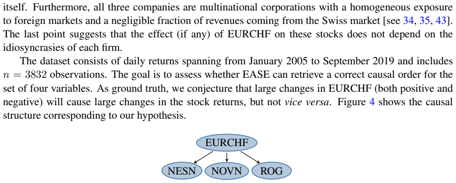
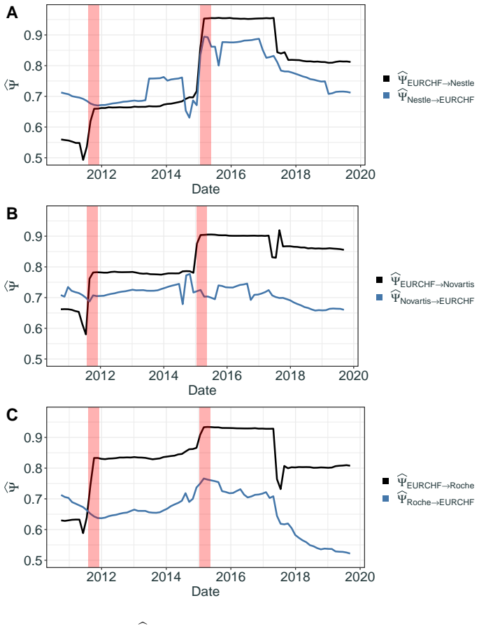
[Section 5.2] The statement that the estimated shape parameters "seem reasonable" because their confidence intervals overlap is informal; the later acknowledgment that NESN and NOVN have slightly lighter tails is more accurate. Consider presenting a more explicit check of the comparability assumption (4) for this dataset.
[Section 4.3] The sentence "However, this does not affect the correctness of the EASE algorithm, on the population level" is immediately qualified by Example 2, where EASE can make mistakes when Γjk = Γkj = 1 for an ancestor-descendant pair. Rephrase to reflect the conditional nature, for example by saying "apart from the case in Example 2".
[Section 3.1] The EASE algorithm description does not specify tie-breaking when multiple nodes attain the minimal score M_i^{(s)}. Adding a sentence that ties are broken arbitrarily would make the algorithm fully deterministic.

Circularity Check

0 steps flagged · score 0.0 of 10

No significant circularity: the causal tail coefficient is defined independently of the target graph, the identifiability theorem is derived in closed form, and the algorithm's correctness follows from that theorem rather than from a fitted parameter or a self-citation chain.

full rationale

The population derivation is self-contained. Definition 1 defines Γjk as a distributional functional, without reference to the underlying DAG; Lemma 1 derives its closed form from the heavy-tailed linear SCM via regular variation (Section 2.1, Eq. (4), and Lemma 3 in Appendix A). Theorem 1 then solves the classification from that closed form (Appendix B.2), and Proposition 1 proves EASE's correctness using only Theorem 1 (Appendix B.4). No parameter is fitted to the target quantity and then renamed a prediction. The threshold k_n is an estimator hyperparameter, not part of the identifiability theorem, and the simulation protocol states that the data used to choose k_n are independent of the evaluation data: 'The simulated data is independent of the data used to choose the best fractional exponent of kn' (Section 5.1.2). The paper's own Section 4.3 explicitly discusses failure modes when noise tails differ, for example Example 3, where a heavier-tailed common ancestor can make Γjk = 1 in the wrong direction; this is an honest boundary of the stated assumptions, not a circular step. Self-citations in the applications, such as Asadi et al. [1] and Engelke and Hitz [12], are dataset and background references and are not load-bearing support for the central theorem. No step in the derivation assumes the conclusion it purports to prove.

Assumptions & free parameters 1 free parameters · 5 assumptions · 0 invented entities

The central claims rest mainly on domain assumptions (common tail index, linear SCM, DAG) and classical EVT results. There are no invented entities. One algorithm hyperparameter, k_n, is tuned in the numerical work.

free parameters (1)

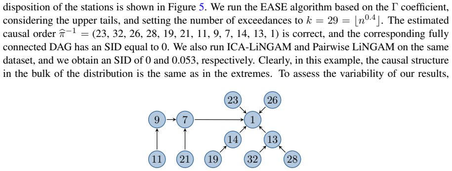
Number of upper order statistics k_n = n^0.4 in simulations; k=10 in financial data; k=29 in river data
Selected by hand from a preliminary simulation (Section 5.1.2, Figure 8). The theory holds for any intermediate sequence, but reported finite-sample performance depends on this choice.

assumptions (5)

domain assumption Noise variables ε_j are independent and regularly varying with comparable tails: P(ε_j>x)∼c_j ℓ(x)x^{-α} for a common α and slowly varying ℓ.
Invoked in Section 2.1, Eq. (4); Lemma 1's closed form and Theorem 1's identifiability collapse the slowly varying terms only under this comparability.
domain assumption Data follow a linear SCM without feedback, with coefficients β_{jk}>0 (Section 2.1) or real β_{jk} with β_{j→k}≠0 for every ancestor relation (Section 4.1).
This model class is the scope of the paper; outside it, the tail coefficient may not encode ancestry.
standard math The induced graph is a directed acyclic graph.
Required for the recursive expansion X_j=∑ β_{h→j} ε_h and for the causal order definition.
domain assumption For the estimator, each marginal density satisfies the von Mises condition and k_n is an intermediate sequence with k_n→∞ and k_n/n→0.
Theorem 2 and Corollaries 1-2 rely on these assumptions via tail empirical process theory.
standard math Standard extreme value facts: max-sum equivalence and regular variation limits (Lemmas 3-6) are used in the proofs.
These are classical results from the cited literature, not derived in the paper.

how reviews work

0 comments

Cite this review

Pith. "Pith review of Causal discovery in heavy-tailed models." pith.science (2026). https://pith.science/paper/GPVU6APL

@misc{pith2026190805097,
  author       = {Pith},
  title        = {Pith review of: Causal discovery in heavy-tailed models},
  year         = {2026},
  howpublished = {\url{https://pith.science/paper/GPVU6APL}},
  note         = {Machine review of arXiv:1908.05097}
}

read the original abstract

Causal questions are omnipresent in many scientific problems. While much progress has been made in the analysis of causal relationships between random variables, these methods are not well suited if the causal mechanisms only manifest themselves in extremes. This work aims to connect the two fields of causal inference and extreme value theory. We define the causal tail coefficient that captures asymmetries in the extremal dependence of two random variables. In the population case, the causal tail coefficient is shown to reveal the causal structure if the distribution follows a linear structural causal model. This holds even in the presence of latent common causes that have the same tail index as the observed variables. Based on a consistent estimator of the causal tail coefficient, we propose a computationally highly efficient algorithm that estimates the causal structure. We prove that our method consistently recovers the causal order and we compare it to other well-established and non-extremal approaches in causal discovery on synthetic and real data. The code is available as an open-access R package.

Figures

Figures reproduced from arXiv: 1908.05097 by the authors.

**Figure 2.** Graphical representation of an SCM with an underlying “diamond” DAG [PITH_FULL_IMAGE:figures/full_fig_p006_2.png] view at source ↗

**Figure 3.** The figure refers to Section 5.1.2. It shows the SID averaged over 50 simulations, for each method, setting, sample size n and dimension p, when the tail index is α = 1.5. Each row of the figure corresponds to one setting. In order, the settings are: (1) Linear SCM; (2) Linear SCM with hidden confounders; (3) Nonlinear SCM; (4) Linear SCM where each variable is transformed to a uniform margin. (EURCHF) induce change… view at source ↗

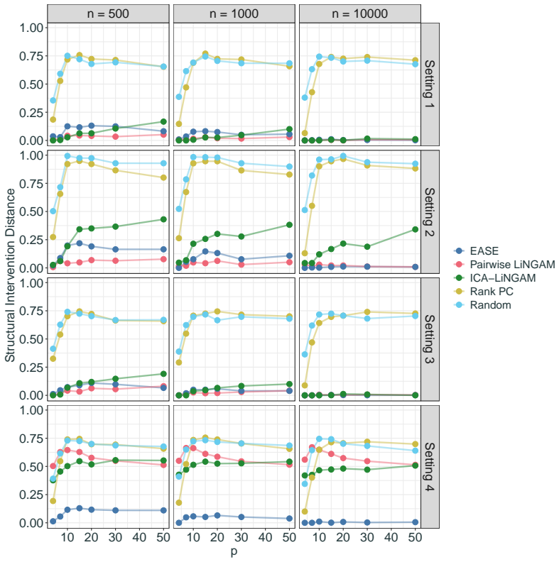
Figures from the paper (14 more)

**Figure 4.** Figure 4: A DAG representing a plausible causal structure among the daily returns of Euro Swiss franc [PITH_FULL_IMAGE:figures/full_fig_p017_4.png]

**Figure 5.** Figure 5: DAG representing the spatial configuration of the stations across the upper Danube basin. [PITH_FULL_IMAGE:figures/full_fig_p019_5.png]

**Figure 6.** Figure 6: DAG G. 1 2 21 213 2134 214 2143 23 231 2314 234 24 3 4 [PITH_FULL_IMAGE:figures/full_fig_p033_6.png]

**Figure 7.** Figure 7: Extremal ancestral search (EASE) for the DAG shown in Figure [PITH_FULL_IMAGE:figures/full_fig_p033_7.png]

**Figure 8.** Figure 8: The figure refers to Section 5.1.2. It shows the structural intervention distance (SID) of the EASE algorithm for different fractional exponents ν ∈ [0.2, 0.7] of kn = bn ν c and different tail indices α ∈ {1.5, 2.5, 3.5}. Each point represents the SID measure averaged…

**Figure 9.** Figure 9: The figure refers to Section 5.3. It shows the robustness of the structural intervention distance (SID) for varying fractional exponents ν ∈ [0.2, 0.7] of kn = bn ν c. Each point represents an average over 50 SID evaluations for the EASE algorithm, after bootstrapping …

**Figure 10.** Figure 10: The figure refers to Section 5.2. It shows the variability of the estimated coefficients Ψb for different fractional exponents ν ∈ [0.2, 0.7] of kn = bn ν c. Each point represents the estimates of Ψb based on the full dataset. The shaded intervals correspond to the 90…

**Figure 11.** Figure 11: The figure refers to Section 5.1.2. It shows the SID averaged over 50 simulations, for each method, setting, sample size n and dimension p, when the tail index is α = 2.5. Each row of the figure corresponds to one setting. In order, the settings are: (1) Linear SCM; (…

**Figure 12.** Figure 12: The figure refers to Section 5.1.2. It shows the SID averaged over 50 simulations, for each method, setting, sample size n and dimension p, when the tail index is α = 3.5. Each row of the figure corresponds to one setting. In order, the settings are: (1) Linear SCM; (…

**Figure 13.** Figure 13: The figure refers to Section 5.3. It represents the map of the upper Danube basin. The plot is created with the ggmap R package developed by Kahle and Wickham [26]. The background is taken from maps.stamen.com. ● ● ● ● ● ● ●● ● ● ●● ● ● ●● ● ● ● ● ● ● ● ● ● ● ● ● ● ● …

**Figure 14.** Figure 14: The figure refers to Section 5.1.2. It shows the base-10 logarithm of the computational time (in seconds) averaged over 10 simulations, for each method, sample size n and dimension p. 39 [PITH_FULL_IMAGE:figures/full_fig_p039_14.png]

**Figure 15.** Figure 15: The figure refers to Section 5.1.2. It shows the average SID of the Rank PC algorithm over 50 simulations for different significance levels of the independent test. For each dimension p we simulate n = 1000 observations from a linear SCM with Student’s-t noise with α …

**Figure 16.** Figure 16: Daily returns of the EURCHF exchange rate. The red sections represent the two major [PITH_FULL_IMAGE:figures/full_fig_p041_16.png]

**Figure 17.** Figure 17: Estimated coefficients Ψb on a rolling window of 1500 days. The threshold used to estimate the coefficient is k = 10. 42 [PITH_FULL_IMAGE:figures/full_fig_p042_17.png]

Discussion (0). Continue with ORCID to comment.

Reference graph

Works this paper leans on

54 extracted references · 53 canonical work pages

[1]

Asadi, A

P. Asadi, A. C. Davison, and S. Engelke. Extremes on river networks. Annals of Applied Statistics, 9(4):2023–2050, 2015

work page 2023
[2]

Basrak and J

B. Basrak and J. Segers. Regularly varying multivariate time series. Stochastic processes and their applications, 119(4):1055–1080, 2009

work page 2009
[3]

K. A. Bollen. Structural Equations with Latent Variables. John Wiley & Sons Inc., New York, NY , USA, 1989

work page 1989
[4]

B ¨uhlmann, J

P. B ¨uhlmann, J. Peters, and J. Ernest. CAM: Causal additive models, high-dimensional order search and penalized regression. Annals of Statistics, 42:2526–2556, 2014

work page 2014
[5]

J. J. Cai, J. H. J. Einmahl, L. de Haan, and C. Zhou. Estimation of the marginal expected shortfall: the mean when a related variable is extreme. Journal of the Royal Statistical Society: Series B (Statistical Methodology), 77:417–442, 2015

work page 2015
[6]

Learning sparse causal models is not np-hard

Tom Claassen, Joris Mooij, and Tom Heskes. Learning sparse causal models is not np-hard. In Proceedings of the Twenty-Ninth Conference on Uncertainty in Artiﬁcial Intelligence (UAI), pages 172–181. ACM Press, 2013

work page 2013
[7]

An Introduction to Statistical Modeling of Extreme Values

Stuart Coles. An Introduction to Statistical Modeling of Extreme Values. Springer, New York, NY , USA, 2001

work page 2001
[8]

P. Comon. Independent component analysis, a new concept? Signal processing, 36(3):287–314, 1994

1994

Show all 54 references

[9]

Multivariate Dependencies: Models, Analysis and In- terpretation, volume 67 of Monographs on Statistics and Applied Probability

David Roxbee Cox and Nanny Wermuth. Multivariate Dependencies: Models, Analysis and In- terpretation, volume 67 of Monographs on Statistics and Applied Probability . CRC Press, Boca Raton, FL, USA, 1996

1996
[10]

de Haan and A

L. de Haan and A. Ferreira. Extreme Value Theory. Springer, New York, NY , USA, 2006

2006
[11]

Embrechts, C

P. Embrechts, C. Kl ¨uppelberg, and T. Mikosch. Modelling Extremal Events: for Insurance and Finance. Springer, New York, NY , USA, 1997

1997
[12]

Engelke and A.S

S. Engelke and A.S. Hitz. Graphical models for extremes. Journal of the Royal Statistical Society: Series B (Statistical Methodology), 82:871–932, 2020. Discussion paper

2020
[13]

Engelke and J

S. Engelke and J. Ivanovs. Sparse structures for multivariate extremes. Annual Review of Statistics and Its Application, 8, 2021. To appear

2021
[14]

Discovering unconfounded causal relationships using linear non-gaussian models

Doris Entner and Patrik O Hoyer. Discovering unconfounded causal relationships using linear non-gaussian models. In Proceedings of the 2010 international conference on New Frontiers in Artiﬁcial Intelligence, pages 181–195. Springer, 2010

2010
[15]

Improved estimation for temporally clustered extremes

Lee Fawcett and David Walshaw. Improved estimation for temporally clustered extremes. Envi- ronmetrics, 18(2):173–188, 2007

2007
[16]

W. Feller. An Introduction to Probability Theory and Its Applications, Volume II . John Wiley & Sons Inc., New York, NY , USA, 1971

1971
[17]

K. J. Forbes and R. Rigobon. No contagion, only interdependence: Measuring stock market co- movements. The Journal of Finance, 57(5):2223–2261, 2002. 43

2002
[18]

Gissibl and C

N. Gissibl and C. Kl ¨uppelberg. Max-linear models on directed acyclic graphs. Bernoulli, 24(4A): 2693–2720, 2018

2018
[19]

Identiﬁability and estimation of re- cursive max-linear models

Nadine Gissibl, Claudia Kl ¨uppelberg, and Steffen Lauritzen. Identiﬁability and estimation of re- cursive max-linear models. Scandinavian Journal of Statistics, 2020. To appear

2020
[20]

Investigating causal relations by econometric models and cross-spectral meth- ods

Clive WJ Granger. Investigating causal relations by econometric models and cross-spectral meth- ods. Econometrica, 37(3):424–438, 1969

1969
[21]

Harris and M

N. Harris and M. Drton. PC algorithm for nonparanormal graphical models. Journal of Machine Learning Research, 14(1):3365–3383, 2013

2013
[22]

A simple general approach to inference about the tail of a distribution

Bruce M Hill. A simple general approach to inference about the tail of a distribution. Annals of Statistics, 3(5):1163–1174, 1975

1975
[23]

P. O. Hoyer, S. Shimizu, A. J. Kerminen, and M. Palviainen. Estimation of causal effects using linear non-gaussian causal models with hidden variables. International Journal of Approximate Reasoning, 49(2):362–378, 2008

2008
[24]

Pairwise likelihood ratios for estimation of non-gaussian structural equation models

Aapo Hyv ¨arinen and Stephen M Smith. Pairwise likelihood ratios for estimation of non-gaussian structural equation models. Journal of Machine Learning Research, 14(Jan):111–152, 2013

2013
[25]

G. W. Imbens and D. B. Rubin. Causal Inference for Statistics, Social, and Biomedical Sciences: An Introduction. Cambridge University Press, New York, NY , USA, 2015

2015
[26]

ggmap: Spatial visualization with ggplot2

David Kahle and Hadley Wickham. ggmap: Spatial visualization with ggplot2. The R Journal, 5 (1):144–161, 2013. URL https://journal.r-project.org/archive/2013-1/kahle-wickham.pdf

2013
[27]

Kalisch, M

M. Kalisch, M. M ¨achler, D. Colombo, M. H. Maathuis, and P. B¨uhlmann. Causal inference using graphical models with the r package pcalg. Journal of Statistical Software, 47(11):1–26, 2012

2012
[28]

Three approaches to the quantitative deﬁnition of information

Andrei Nikolaevich Kolmogorov. Three approaches to the quantitative deﬁnition of information. International journal of computer mathematics, 2(1-4):157–168, 1968

1968
[29]

S. L. Lauritzen. Graphical models. Oxford Statistical Science Series. A Clarendon Press Publica- tion. Oxford University Press, New York, NY , USA, 1996

1996
[30]

S. L. Lauritzen, A. P. Dawid, B. N. Larsen, and H. G. Leimer. Independence properties of directed markov ﬁelds. Networks, 20(5):491–505, 1990

1990
[31]

Linda Mhalla, Valrie Chavez-Demoulin, and Debbie J. Dupuis. Causal mechanism of extreme river discharges in the upper danube basin network. Journal of the Royal Statistical Society: Series C (Applied Statistics), 69(4):741–764, 2020

2020
[32]

Misra and E

N. Misra and E. E. Kuruoglu. Stable graphical models. Journal of Machine Learning Research, 17(168):1–36, 2016

2016
[33]

Naveau, A

P. Naveau, A. Ribes, F. Zwiers, A. Hannart, A. Tuel, and P. Yiou. Revising return periods for record events in a climate event attribution context. Journal of Climate, 31(9):3411–3422, 2018

2018
[34]

Financial statements 2019

Nestl ´e. Financial statements 2019. Online release, page 89, 2019

2019
[35]

Annual report 2019

Novartis. Annual report 2019. Online release, pages F–25–26, 2019

2019
[36]

J. Pearl. Causality: Models, Reasoning, and Inference . Cambridge University Press, New York, NY , USA, 2nd edition, 2009. 44

2009
[37]

Peters and P

J. Peters and P. B ¨uhlmann. Structural intervention distance for evaluating causal graphs. Neural computation, 27(3):771–799, 2015

2015
[38]

Peters, D

J. Peters, D. Janzing, and B. Sch ¨olkopf. Elements of Causal Inference: Foundations and Learning Algorithms. MIT Press, Cambridge, MA, USA, 2017

2017
[39]

Identiﬁability of gaussian structural equation models with equal error variances

Jonas Peters and Peter B ¨uhlmann. Identiﬁability of gaussian structural equation models with equal error variances. Biometrika, 101(1):219–228, 2014

2014
[40]

Detecting the direction of causal time series

Jonas Peters, Dominik Janzing, Arthur Gretton, and Bernhard Sch ¨olkopf. Detecting the direction of causal time series. In Proceedings of the 26th International Conference on Machine Learning (ICML), pages 801–808. ACM Press, 2009

2009
[41]

Causal discovery with continuous additive noise models.Journal of Machine Learning Research, 15(1):2009–2053, 2014

Jonas Peters, Joris M Mooij, Dominik Janzing, and Bernhard Sch ¨olkopf. Causal discovery with continuous additive noise models.Journal of Machine Learning Research, 15(1):2009–2053, 2014

2009
[42]

S. I. Resnick. Extreme Values, Regular Variation and Point Processes. Springer, New York, NY , USA, 1987

1987
[43]

Finance report 2019

Roche. Finance report 2019. Online release, page 160, 2019

2019
[44]

J. C. Rodriguez. Measuring ﬁnancial contagion: A copula approach. Journal of Empirical Finance, 14(3):401–423, 2007

2007
[45]

Limit theorems for sampling from ﬁnite populations

Bengt Ros ´en. Limit theorems for sampling from ﬁnite populations. Arkiv f¨or Matematik, 5:383– 424, 1965

1965
[46]

S. I. Seneviratne, T. Corti, E. L. Davin, M. Hirschi, E. B. Jaeger, I. Lehner, B. Orlowsky, and A. J. Teuling. Investigating soil moisture–climate interactions in a changing climate: A review. Earth-Science Reviews, 99(3-4):125–161, 2010

2010
[47]

Shimizu, P

S. Shimizu, P. O. Hoyer, A. Hyv¨arinen, and A. Kerminen. A linear non-gaussian acyclic model for causal discovery. Journal of Machine Learning Research, 7(Oct):2003–2030, 2006

2003
[48]

Shimizu, T

S. Shimizu, T. Inazumi, Y . Sogawa, A. Hyv ¨arinen, Y . Kawahara, T. Washio, P. O. Hoyer, and K. Bollen. Directlingam: A direct method for learning a linear non-gaussian structural equation model. Journal of Machine Learning Research, 12(Apr):1225–1248, 2011

2011
[49]

Regional estimation from spatially dependent data

Richard L Smith. Regional estimation from spatially dependent data. 1990. Unpublished

1990
[50]

Spirtes, C

P. Spirtes, C. N. Glymour, and Scheines. Causation, Prediction, and Search . MIT press, Cam- bridge, MA, USA, 2000

2000
[51]

Tashiro, S

T. Tashiro, S. Shimizu, A. Hyv ¨arinen, and T. Washio. Parcelingam: A causal ordering method robust against latent confounders. Neural Computation, 26(1):57–83, 2014

2014
[52]

Causal discovery with unobserved confounding and non- gaussian data

Y Samuel Wang and Mathias Drton. Causal discovery with unobserved confounding and non- gaussian data. arXiv preprint arXiv:2007.11131, 2020

2007 arXiv
[53]

J. Zhang. Causal reasoning with ancestral graphs. Journal of Machine Learning Research, 9(Jul): 1437–1474, 2008

2008
[54]

N. Zou, S. V olgushev, and A. B¨ucher. Multiple block sizes and overlapping blocks for multivariate time series extremes. Annals of Statistics. To appear. 45

Pith tools

Reviewed August 14, 2026 · model on record in the stance chip above.

[1] [1]

Asadi, A

P. Asadi, A. C. Davison, and S. Engelke. Extremes on river networks. Annals of Applied Statistics, 9(4):2023–2050, 2015

work page 2023

[2] [2]

Basrak and J

B. Basrak and J. Segers. Regularly varying multivariate time series. Stochastic processes and their applications, 119(4):1055–1080, 2009

work page 2009

[3] [3]

K. A. Bollen. Structural Equations with Latent Variables. John Wiley & Sons Inc., New York, NY , USA, 1989

work page 1989

[4] [4]

B ¨uhlmann, J

P. B ¨uhlmann, J. Peters, and J. Ernest. CAM: Causal additive models, high-dimensional order search and penalized regression. Annals of Statistics, 42:2526–2556, 2014

work page 2014

[5] [5]

J. J. Cai, J. H. J. Einmahl, L. de Haan, and C. Zhou. Estimation of the marginal expected shortfall: the mean when a related variable is extreme. Journal of the Royal Statistical Society: Series B (Statistical Methodology), 77:417–442, 2015

work page 2015

[6] [6]

Learning sparse causal models is not np-hard

Tom Claassen, Joris Mooij, and Tom Heskes. Learning sparse causal models is not np-hard. In Proceedings of the Twenty-Ninth Conference on Uncertainty in Artiﬁcial Intelligence (UAI), pages 172–181. ACM Press, 2013

work page 2013

[7] [7]

An Introduction to Statistical Modeling of Extreme Values

Stuart Coles. An Introduction to Statistical Modeling of Extreme Values. Springer, New York, NY , USA, 2001

work page 2001

[8] [8]

P. Comon. Independent component analysis, a new concept? Signal processing, 36(3):287–314, 1994

1994