REVIEW 3 major objections 9 minor 82 references
Bayesian spatial modelling framework for assessing residential flood risk in property insurance
T0 review · 3 major / 9 minor · reviewed 2026-07-09 · glm-5.2
Pith's one-line read Continuous spatial model beats zone-based flood insurance pricing
desk verdict First point-referenced SPDE for flood insurance; solid applied work with a real fairness concern in the model comparison read the letter →
The pith
A machine-rendered reading of the paper's core claim, the machinery that carries it, and where it could break.
The reading
What carries the argument
INLA-SPDE: a Bayesian inference method combining Integrated Nested Laplace Approximation with a Stochastic Partial Differential Equation representation of a Matérn Gaussian random field, allowing spatial dependence to be modelled on a continuous surface discretised via a triangulated mesh rather than on fixed geographic zones.
What would settle it
If adding an explicit temporal correlation structure to the SPDE model substantially reduces the estimated spatial range or the marginal contribution of the spatial field to predictive metrics, the spatial gains reported here would be partially attributable to unmodelled temporal dependence rather than genuine spatial structure.
Extended reading notes
Core claim
A continuously indexed spatial random field (SPDE) fitted at the building level captures sub-municipal flood risk variation that both GLMs and areal Bayesian models miss, yielding materially better occurrence prediction and premium allocation across a large national insurance portfolio.
Load-bearing premise
The model treats each policy-year observation as temporally independent and does not explicitly model temporal correlation. If the same buildings flood repeatedly across years, the spatial random field may absorb temporal structure, inflating the apparent contribution of spatial dependence to predictive performance.
Editorial extensions
If this is right
- Insurers using zone-based spatial pricing may be systematically underpricing high-risk clusters within nominally safe municipalities, creating adverse selection exposure visible only at sub-municipal resolution.
- Regulatory flood hazard maps (TRI, PPRI) partially overlap with model-identified high-risk areas but miss localised hotspots, suggesting that continuous statistical models can complement or challenge institutional hazard assessments.
- The finding that severity gains from spatial modelling are limited implies that insurers can focus spatial refinement on frequency modelling and use simpler structures for cost prediction, reducing computational burden.
- Bayesian posterior upper-tail quantiles enable identification of buildings with credible extreme-event risk even without historical claims, supporting proactive underwriting in data-sparse but structurally exposed locations.
Editorial analysis
A structured set of objections, weighed in public.
Referee Report
Summary. This manuscript applies a point-referenced Bayesian spatial modelling framework to residential flood insurance risk, comparing a benchmark GLM against Bayesian GAMs with discrete areal random effects (IID, iCAR, BYM) and a continuously indexed Matérn Gaussian random field via the SPDE approach, all estimated with INLA. Using a large French insurance portfolio (968k properties, 4.9M policy-years, ~10,800 flood claims) enriched with high-resolution environmental and meteorological covariates, the authors evaluate occurrence and severity models on a temporally held-out validation set. They find that spatial random effects substantially improve occurrence prediction, that the SPDE formulation outperforms areal models, and that severity gains from spatial structure are marginal. A pure premium analysis and Bayesian uncertainty quantification illustrate operational relevance for pricing and tail-risk assessment.
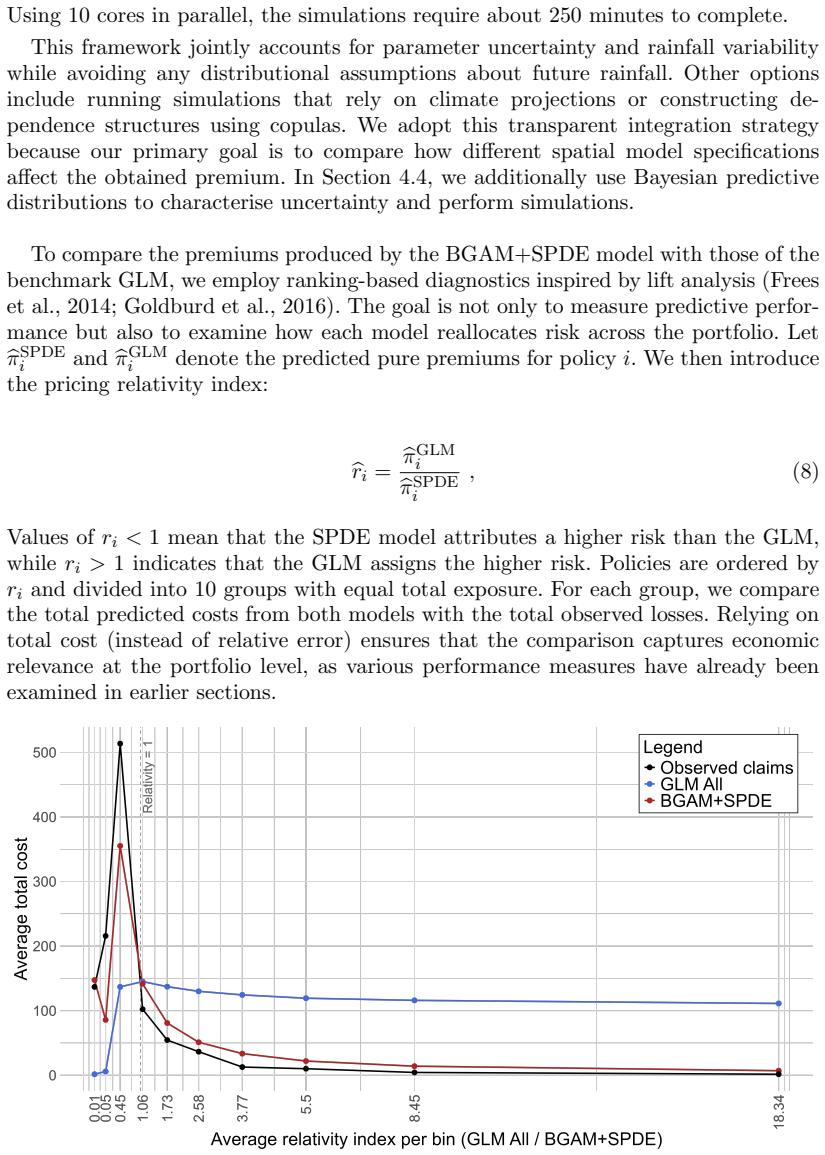
Significance. The paper tackles a practically important problem in actuarial spatial modelling and the application of INLA-SPDE to a national-scale flood insurance portfolio is a genuine methodological contribution. The systematic model comparison (Table 2, Table 3) across multiple metrics (WAIC, Gini, CSI) on held-out data is commendable, as is the use of PC priors for the Matérn parameters (§3.4) calibrated via domain knowledge rather than validation outcomes. The pure premium analysis (Table 4, Figure 6) and the Bayesian uncertainty quantification (§4.4) provide concrete, falsifiable demonstrations of the framework's operational value. The intra-municipal case study (Figure 4) effectively illustrates the sub-municipal differentiation that motivates the continuous spatial approach.
major comments (3)
- §3.3 states that SPDE mesh hyperparameters are 'chosen to maximise predictive performance under the constraint that computation time does not exceed that of the discrete areal models.' If this selection used the validation set, the SPDE's Table 2 metrics are optimistically biased relative to the untuned areal models, which use fixed administrative boundaries with no comparable optimisation. The paper must clarify whether mesh tuning used the validation set or a separate tuning partition. If validation data were used for mesh selection, the comparison in Tables 2–3 is not on equal footing and the central claim of SPDE superiority is compromised. At minimum, the sensitivity checks mentioned in §3.4 ('random splits, geographic validation, and shorter training windows produced similar model rankings') should be quantified and reported, as geographic hold-out would directly test whether theSP
- §3.1: 'the temporal dimension is not explicitly modelled; instead, policy-year observations are treated as independent.' The validation set is a temporally held-out sample of recent policy years (§3.4), meaning the same buildings appear in both training and validation. The SPDE's continuous spatial field with its locally refined mesh (12,613 nodes nationally) can memorise building-specific or micro-location patterns from training-year claims and apply them at the same locations in validation. The iCAR/BYM models, constrained to a single municipality-level effect, cannot exploit this. The SPDE's advantage may thus partly reflect temporal persistence at specific locations rather than genuine spatial structure. A building-level random effect or a geographic hold-out validation (training on one region, predicting another) would help disentangle these mechanisms. The paper should at leastdisc
- Table 3: the severity model gains are marginal (RMSE 8835 → 8656, a 2% improvement) and the Gini increase from 24.7% to 26.8% is modest. The abstract states that 'gains in severity prediction are more limited,' which is accurate, but the conclusion (§5) still lists the SPDE as offering 'the best balance between predictive performance, computational cost, and interpretability' without separately qualifying the severity component. Given that the pure premium (§4.3) combines occurrence and severity, the limited severity improvement should be more explicitly acknowledged in the overall assessment, and the paper should clarify whether the pure premium gains (Table 4) are driven almost entirely by the occurrence model.
minor comments (9)
- §3.4: the PC prior thresholds (σ₀, ρ₀) are described as 'determined using domain knowledge and the spatial scale of the data' but their specific values are not reported. Please state the actual values used.
- Table 2: the CSI threshold is selected to maximise CSI on the training set, but the threshold value itself is not reported. Please include it.
- Figure 3 caption: 'BGAM+SPDE and GLM flood probability of occurrence predictions on the validation set averaged by municipality across policy-years.' It would help to also show the iCAR predictions at this scale, or explicitly state why the discrete and continuous models are 'indistinguishable' at municipal aggregation.
- §4.3, Eq. (7): the Monte Carlo integration uses R=1000 rainfall scenarios and S=100 posterior draws. Please clarify whether the rainfall scenarios are sampled with replacement from observed years and whether the same scenario set is used across all policies.
- Table 4: the 'Bottom 10%' and 'Bottom 5%' rows appear to be nested subsets but this is not explicitly stated. A footnote clarifying the relationship between these segments would aid interpretation.
- §4.4: the posterior predictive check reports a simulated median of 11,007 claims nationally vs 10,800 observed, but no interval or calibration metric is given for this comparison beyond the 97.5% quantile. A simple posterior predictive p-value or interval would strengthen the calibration claim.
- The self-citation (Moriah et al., 2026) is used for data construction details and variable definitions. Given that this appears to be a companion or predecessor paper, please ensure the present manuscript is self-contained regarding the definitions of MILRE and ann MILRE (Appendix A helps but references the companion paper for methodology).
- Minor typo: §1.2, 'Besag-York-Mollié' is sometimes written 'Besag-York-Mollie' (e.g., abstract of the full text vs. §3.2.1). Please standardise.
- Figure 2 caption states 1,512 nodes for Occitanie, while §3.3 states 12,613 nodes nationally. It would be useful to note the proportion of national claims or exposure falling in the locally refined areas.
Simulated Author's Rebuttal
We thank the referee for a careful and constructive report. The three major comments raise legitimate concerns about (1) whether mesh tuning on the validation set biases the SPDE comparison, (2) whether the SPDE's advantage reflects temporal persistence at building locations rather than genuine spatial structure, and (3) whether the severity gains are overstated in the conclusion. We address each below and commit to revisions in all three areas.
read point-by-point responses
-
Referee: §3.3 states that SPDE mesh hyperparameters are 'chosen to maximise predictive performance under the constraint that computation time does not exceed that of the discrete areal models.' If this selection used the validation set, the SPDE's Table 2 metrics are optimistically biased relative to the untuned areal models. The paper must clarify whether mesh tuning used the validation set or a separate tuning partition. At minimum, the sensitivity checks mentioned in §3.4 should be quantified and reported, as geographic hold-out would directly test whether the SPDE advantage holds.
Authors: The referee raises a valid and important concern. We must be transparent: the mesh hyperparameters were selected using the validation set, not a separate tuning partition. This means the SPDE model did receive a form of tuning that the areal models, which use fixed administrative boundaries, did not. We agree this creates a potential optimistic bias in the head-to-head comparison in Tables 2–3. We will address this in two ways. First, we will revise §3.3 to state explicitly and honestly that mesh selection used the validation set, and we will add a caveat acknowledging the resulting asymmetry. Second, we will quantify and report the sensitivity checks already mentioned in §3.4. Specifically, we conducted geographic hold-out validation (training on one region, predicting another) and random-split validation during our analysis. We will add a table or appendix reporting the model rankings under these alternative partitions. We can state now that the geographic hold-out results preserved the SPDE's relative advantage over areal models, though with attenuated margins, and we will report the exact figures. If, upon re-examination, the geographic hold-out results are less conclusive than we recalled, we will report that honestly and adjust the strength of our claims accordingly. revision: yes
-
Referee: §3.1: the temporal dimension is not explicitly modelled; policy-year observations are treated as independent. The validation set is temporally held-out, meaning the same buildings appear in both training and validation. The SPDE's continuous spatial field with its locally refined mesh can memorise building-specific or micro-location patterns from training-year claims and apply them at the same locations in validation. The iCAR/BYM models cannot exploit this. The SPDE's advantage may partly reflect temporal persistence at specific locations rather than genuine spatial structure. A building-level random effect or a geographic hold-out validation would help disentangle these mechanisms.
Authors: This is a thoughtful observation and we acknowledge the mechanism the referee describes is real. Because the same buildings appear in both training and validation years, and because the SPDE mesh is locally refined in dense areas, the continuous spatial field can in principle capture location-specific persistent effects that the municipality-level areal models cannot. This is partly by design—the SPDE is meant to capture fine-scale spatial structure that persists over time—but the referee is right that it confounds genuine spatial smoothing with temporal persistence at fixed locations. We cannot fully resolve this with the current data and model specification: adding a building-level random effect would be computationally prohibitive at 968k properties and would conflate spatial structure with individual heterogeneity in a different way. However, we can partially address the concern. The geographic hold-out validation we mention in §3.4 trains on one region and predicts another, which by construction uses different buildings and thus eliminates the memorisation mechanism. We will report these results explicitly. Additionally, we will add a paragraph in §5 discussing this limitation transparently, noting that the SPDE's advantage in the temporal hold-out setting may partly reflect temporal persistence at specific locations, and that the geographic hold-out results (which we will quantify) provide a more conservative test. We cannot claim to fully disentangle the two mechanisms, and we will not present the SPDE advantage as solely due to spatial structure without this qualification. revision: partial
-
Referee: Table 3: the severity model gains are marginal (RMSE 8835 → 8656, a 2% improvement) and the Gini increase from 24.7% to 26.8% is modest. The conclusion (§5) still lists the SPDE as offering 'the best balance between predictive performance, computational cost, and interpretability' without separately qualifying the severity component. Given that the pure premium combines occurrence and severity, the limited severity improvement should be more explicitly acknowledged in the overall assessment, and the paper should clarify whether the pure premium gains are driven almost entirely by the occurrence model.
Authors: The referee is correct on both points. The severity gains are indeed marginal—a 2% RMSE improvement is small—and the conclusion as written does not adequately qualify this. We will revise §5 to explicitly state that the SPDE's advantage is concentrated in the occurrence model, while severity gains are limited and may not justify the added complexity for practitioners focused solely on cost prediction. Regarding the pure premium: yes, the gains in Table 4 and Figure 6 are driven almost entirely by the occurrence component. The severity model contributes nearly identical predictions across specifications, so the improvement in premium allocation comes from better occurrence probability estimation. We will add a sentence to §4.3 stating this directly. We will also soften the conclusion's claim about 'the best balance' to specify that this assessment applies primarily to the occurrence model and the pure premium through the occurrence channel, not to standalone severity prediction. revision: yes
Circularity Check
No significant circularity found; derivation is self-contained against external benchmarks
full rationale
The paper compares standard, well-established model specifications (GLM, BGAM with IID/iCAR/BYM/SPDE spatial effects) on a temporally held-out validation set using conventional metrics (WAIC, Gini, CSI, RMSE). No model is defined in terms of the target predictions. The SPDE spatial field (Eq. 6) is defined via the Lindgren et al. (2011) SPDE representation of a Matérn GRF — an external, widely cited methodological result, not a self-citation. PC priors (§3.4) are set using domain knowledge (tail probabilities 0.05, thresholds from spatial scale of data), not fitted to validation outcomes. The pure premium (Eq. 7) is a standard frequency-severity decomposition with Monte Carlo integration over rainfall scenarios. The self-citation to Moriah et al. (2026) provides the data pipeline and covariate definitions (MILRE, annMILRE, tail weight cluster), but these are fully described in the present paper (Table 1, Appendix A) and are not load-bearing for the central methodological claim about SPDE vs. areal model performance. The mesh hyperparameter tuning ('chosen to maximise predictive performance,' §3.3) raises a fairness concern about validation-set optimism for the SPDE model relative to untuned areal models, but this is a methodological design issue, not circularity: the SPDE predictions are still produced by Bayesian inference on training data, not by construction equivalent to the validation outcomes. No step in the derivation chain reduces to its inputs by definition or by self-citation.
Assumptions & free parameters
free parameters (8)
- Matérn marginal SD (σ)
- Matérn spatial range (ρ)
- Matérn smoothness (ν)
- Mesh max edge (interior)
- Mesh max edge (outer)
- Mesh cutoff (min node separation)
- Spline knot positions and counts
- CSI threshold
assumptions (4)
- domain assumption Policy-year observations are conditionally independent given covariates and spatial effects (temporal correlation ignored).
- domain assumption At most one flood claim per policy-year justifies Bernoulli likelihood for occurrence.
- domain assumption Gamma distribution with log link adequately models conditional claim severity.
- domain assumption The SPDE Matérn approximation on the chosen mesh adequately represents the true continuous Gaussian random field.
Cite this review
Pith. "Pith review of Bayesian spatial modelling framework for assessing residential flood risk in property insurance." pith.science (2026). https://pith.science/paper/GRJQJP2F
@misc{pith2026260707609,
  author       = {Pith},
  title        = {Pith review of: Bayesian spatial modelling framework for assessing residential flood risk in property insurance},
  year         = {2026},
  howpublished = {\url{https://pith.science/paper/GRJQJP2F}},
  note         = {Machine review of arXiv:2607.07609}
}
read the original abstract
Spatial heterogeneity in insurance risk modelling is often represented using coarse areal structures, which can obscure fine-scale patterns critical for accurate risk assessment. This study introduces a point-referenced Bayesian framework to model claim occurrence and severity at the policyholder level, avoiding reliance on predefined geographic aggregation. Drawing on a large French insurance portfolio combined with high-resolution environmental variables, rainfall records, and institutional hazard maps, we compare a benchmark GLM with several discrete Bayesian specifications, including independent random effects, intrinsic conditional autoregressive (iCAR) and Besag-York-Mollie (BYM) models, and a continuously indexed Gaussian random field constructed using the stochastic partial differential equation (SPDE) approach. Inference is performed using Integrated Nested Laplace Approximation (INLA), enabling efficient estimation of latent spatial fields and non-linear covariate effects. Our results show that accounting for spatial dependence substantially improves occurrence modelling, while gains in severity prediction are more limited. The SPDE formulation further outperforms areal models by capturing sub-municipal risk gradients and reducing artefacts induced by arbitrary geographic partitioning. By conditioning on detailed building-level attributes, we isolate the contribution of latent spatial effects, refine the interpretation of observed covariates, and improve the allocation of risk premiums across the portfolio. In addition to enhanced predictive performance, the framework provides coherent uncertainty quantification and supports tail-risk assessment. To our knowledge, this is the first application of point-referenced SPDE models to flood insurance, offering a scalable statistical alternative for pricing and managing risks with strong spatial structure.
Figures


Figures from the paper (5 more)




Reference graph
Works this paper leans on
-
[1]
Uses of catastrophe model output (2018)
American Academy of Actuaries, Extreme Events and Property Lines Committee. Uses of catastrophe model output (2018). Actuary . org
work page 2018
-
[2]
André, C., Monfort, D., Bouzit, M., & Vinchon, C. (2013). Contribution of insurance data to cost assessment of coastal flood damage to residential buildings: insights gained from Johanna (2008) and Xynthia (2010) storm events. Natural Hazards and Earth System Sciences, 13(8), 2003-2012
work page 2013
-
[3]
Assunção, R., Costa, M. A., Prates, M. O., & Silva e Silva, L. S. G. (2014). Spatial analysis. In A. Charpentier (Ed.), Computational actuarial science with R (pp. 207-256). Chapman & Hall
work page 2014
-
[4]
France Assureurs. (2021). Impact du changement climatique sur l'assurance à l'horizon 2050. Étude FA
work page 2021
-
[5]
A., Riebler, A., Bolin, D., Illian, J.,
Bakka, H., Rue, H., Fuglstad, G. A., Riebler, A., Bolin, D., Illian, J., ... & Lindgren, F. (2018). Spatial modelling with R‐INLA: A review. Wiley Interdisciplinary Reviews: Computational Statistics, 10(6), e1443
work page 2018
-
[6]
B., Trefalt, S., Martius, O., Weingartner, R., Mosimann, M., Röthlisberger, V., & Zischg, A
Bernet, D. B., Trefalt, S., Martius, O., Weingartner, R., Mosimann, M., Röthlisberger, V., & Zischg, A. P. (2019). Characterizing precipitation events leading to surface water flood damage over large regions of complex terrain. Environmental Research Letters, 14(6), 064010
work page 2019
-
[7]
Besag, J., York, J., & Mollié, A. (1991). Bayesian image restoration, with two applications in spatial statistics. Annals of the institute of statistical mathematics, 43(1), 1-20
work page 1991
-
[8]
Besag, J. (1974). Spatial interaction and the statistical analysis of lattice systems. Journal of the Royal Statistical Society: Series B (Methodological), 36(2), 192-225
work page 1974
Show all 82 references
-
[9]
and Wilkins, W.R
Boa, J.M., Underwood, A.M. and Wilkins, W.R. (2006). Casualty Actuarial Society. In Encyclopedia of Actuarial Science (eds J.L. Teugels, B. Sundt and J. Lemaire)
2006
-
[10]
Boskov, M., & Verrall, R. J. (1994). Premium rating by geographic area using spatial models. ASTIN Bulletin: The Journal of the IAA, 24(1), 131-143
1994
-
[11]
Boudreault, M., & Ojeda, A. (2022). Ratemaking territories and adverse selection for flood insurance. Insurance: Mathematics and Economics, 107, 349-360
2022
-
[12]
Centre Européen de Prévention du Risque Inondation. (2022). French implementation of the European Flood Directive. CEPRI. https://cepri.net/les-outils-a-votre-disposition/les-lois-et-le-risque-inondation/loi-grenelle-2/
2022
-
[13]
Chatelain, P., & Loisel, S. (2021). Subsidence and household insurances in France: geolocated data and insurability
2021
-
[14]
S., Li, Q., Li, G., & Auld, H
Cheng, C. S., Li, Q., Li, G., & Auld, H. (2012). Climate change and heavy rainfall-related water damage insurance claims and losses in Ontario, Canada. Journal of Water Resource and Protection, 4(2), 49-62
2012
-
[15]
Denuit, M., Sznajder, D., & Trufin, J. (2019). Model selection based on Lorenz and concentration curves, Gini indices and convex order. Insurance: Mathematics and Economics, 89, 128-139
2019
-
[16]
Denuit, M., & Lang, S. (2004). Non-life rate-making with Bayesian GAMs. Insurance: Mathematics and Economics, 35(3), 627-647
2004
-
[17]
Denuit, M., Charpentier, A., & Bébéar, C. (2004). Mathématiques de l'Assurance Non-Vie. Tome I: Principes Fondamentaux de Théorie du Risque
2004
-
[18]
K., & Di Rattalma, A
Dimakos, X. K., & Di Rattalma, A. F. (2002). Bayesian premium rating with latent structure. Scandinavian Actuarial Journal, 2002(3), 162-184
2002
-
[19]
Dorfman, R. (1979). A formula for the Gini coefficient. The review of economics and statistics, 146-149
1979
-
[20]
DRIEAT (Direction régionale et interdépartementale de l'environnement, de l'aménagement et des transports). (2023). Plan de prévention des risques inondation. Ministère de la Transition écologique. https://www.ecologie.gouv.fr/politiques-publiques/prevention-inondations
2023
-
[21]
Dutta, S., van Niekerk, J., & Rue, H. (2025). Scalable skewed Bayesian inference for latent Gaussian models. arXiv preprint arXiv:2502.19083
2025 arXiv
-
[22]
Muñoz Sabater, J. (2011). ERA5-Land hourly data from 1950 to present. Copernicus Climate Change Service (C3S) Climate Data Store (CDS)
2011
-
[23]
Emanuelsson, P. (2011). Construction of rating territories for water-damage claims (Doctoral dissertation, Stockholm University)
2011
-
[24]
Ferkingstad, E., & Rue, H. (2015). Improving the INLA approach for approximate Bayesian inference for latent Gaussian models
2015
-
[25]
Impact du changement climatique sur l'assurance \`a l'horizon 2050
France Assureurs (2021). Impact du changement climatique sur l'assurance \`a l'horizon 2050. \'Etude FA
2021
-
[26]
W., Meyers, G., & Cummings, A
Frees, E. W., Meyers, G., & Cummings, A. D. (2014). Insurance ratemaking and a Gini index. Journal of Risk and Insurance, 81(2), 335-366
2014
-
[27]
A., Simpson, D., Lindgren, F., & Rue, H
Fuglstad, G. A., Simpson, D., Lindgren, F., & Rue, H. (2019). Constructing priors that penalize the complexity of Gaussian random fields. Journal of the American Statistical Association, 114(525), 445-452
2019
-
[28]
Gaedke-Merzhäuser, L., Krainski, E., Janalik, R., Rue, H., & Schenk, O. (2023). Integrated nested laplace approximations for large-scale spatial-temporal bayesian modelling. arXiv preprint arXiv:2303.15254
2023 arXiv
-
[29]
Base nationale de Gestion ASsistée des Procédures Administratives relatives aux Risques (GASPAR)
GASPAR, Ministère de la Transition écologique. Base nationale de Gestion ASsistée des Procédures Administratives relatives aux Risques (GASPAR). Portail data.gouv. ://www.data.gouv.fr/fr/datasets/base-nationale-de-gestion-assistee-des-procedures-administratives-relatives-aux-r...
-
[30]
Gelman, A., Hwang, J., & Vehtari, A. (2014). Understanding predictive information criteria for Bayesian models. Statistics and computing, 24(6), 997-1016
2014
-
[31]
Goldburd, M., Khare, A., Tevet, D., & Guller, D. (2016). Generalized linear models for insurance rating. Casualty Actuarial Society, CAS Monographs Series, 5, 77
2016
-
[32]
Gradeci, K., Labonnote, N., Sivertsen, E., & Time, B. (2019). The use of insurance data in the analysis of Surface Water Flood events-A systematic review. Journal of Hydrology, 568, 194-206
2019
-
[33]
Grahn, T., & Nyberg, R. (2014). Damage assessment of lake floods: Insured damage to private property during two lake floods in Sweden 2000/2001. International Journal of Disaster Risk Reduction, 10, 305-314
2014
-
[34]
Gschlößl, S., & Czado, C. (2007). Spatial modelling of claim frequency and claim size in non-life insurance. Scandinavian Actuarial Journal, 2007(3), 202-225
2007
-
[35]
(2009, October)
Gu, Q., Zhu, L., & Cai, Z. (2009, October). Evaluation measures of the classification performance of imbalanced data sets. In International symposium on intelligence computation and applications (pp. 461-471). Berlin, Heidelberg: Springer Berlin Heidelberg
2009
-
[36]
Guo, H., & Viktor, H. L. (2004). Learning from imbalanced data sets with boosting and data generation: the databoost-im approach. ACM Sigkdd Explorations Newsletter, 6(1), 30-39
2004
-
[37]
He, H., & Garcia, E. A. (2009). Learning from imbalanced data. IEEE Transactions on knowledge and data engineering, 21(9), 1263-1284
2009
-
[38]
B., Sørbye, S
Illian, J. B., Sørbye, S. H., & Rue, H. (2012). A toolbox for fitting complex spatial point process models using integrated nested Laplace approximation (INLA)
2012
-
[39]
Insee analyses Occitanie
Institut National de Statistiques et des Etudes Economiques (2024). Insee analyses Occitanie. Self-Published Report. Retrieved from https://www.insee.fr/fr/statistiques/8264502
2024
-
[40]
Japkowicz, N. (2013). Assessment metrics for imbalanced learning. Imbalanced learning: Foundations, algorithms, and applications, 187-206
2013
-
[41]
A., Cohn, J
Jeni, L. A., Cohn, J. F., & De La Torre, F. (2013, September). Facing imbalanced data--recommendations for the use of performance metrics. In 2013 Humaine association conference on affective computing and intelligent interaction (pp. 245-251). IEEE
2013
-
[42]
Jennings, P. J. (2008). Using cluster analysis to define geographical rating territories. Applying Multivariate Statistical Models, 34
2008
-
[43]
Jørgensen, B., & Paes De Souza, M. C. (1994). Fitting Tweedie's compound Poisson model to insurance claims data. Scandinavian Actuarial Journal, 1994(1), 69-93
1994
-
[44]
Kaźmierczak, A., & Cavan, G. (2011). Surface water flooding risk to urban communities: Analysis of vulnerability, hazard and exposure. Landscape and urban planning, 103(2), 185-197
2011
-
[45]
& Rue, H
Krainski, E., Gómez-Rubio, V., Bakka, H., Lenzi, A., Castro-Camilo, D., Simpson, D., ... & Rue, H. (2018). Advanced spatial modelling with stochastic partial differential equations using R and INLA. Chapman and Hall/CRC
2018
-
[46]
Legrand, J., Naveau, P., & Oesting, M. (2025). Evaluation of binary classifiers for asymptotically dependent and independent extremes. Journal of the American Statistical Association, 1-19
2025
-
[47]
L., & Opitz, T
Legrand, J., Pimont, F., Dupuy, J. L., & Opitz, T. (2024). Bayesian spatiotemporal modelling of wildfire occurrences and sizes for projections under climate change. Computo
2024
-
[48]
Lindgren, F., Rue, H., & Lindström, J. (2011). An explicit link between Gaussian fields and Gaussian Markov random fields: the stochastic partial differential equation approach. Journal of the Royal Statistical Society Series B: Statistical Methodology, 73(4), 423-498
2011
-
[49]
Lyubchich, V., & Gel, Y. R. (2017). Can we weather proof our insurance?. Environmetrics, 28(2), e2433
2017
-
[50]
Martínez-Gomariz, E., Forero-Ortiz, E., Russo, B., Locatelli, L., Guerrero-Hidalga, M., Yubero, D., & Castan, S. (2021). A novel expert opinion-based approach to compute estimations of flood damage to property in dense urban environments. Barcelona case study. Journal of Hydro...
2021
-
[51]
Merz, B., Kreibich, H., & Lall, U. (2013). Multi-variate flood damage assessment: a tree-based data-mining approach. Natural Hazards and Earth System Sciences, 13(1), 53-64
2013
-
[52]
Merz, B., Kreibich, H., Thieken, A., & Schmidtke, R. (2004). Estimation uncertainty of direct monetary flood damage to buildings. Natural Hazards and Earth System Sciences, 4(1), 153-163
2004
-
[53]
Mobini, S., Nilsson, E., Persson, A., Becker, P., & Larsson, R. (2021). Analysis of pluvial flood damage costs in residential buildings-A case study in Malmö. International Journal of Disaster Risk Reduction, 62, 102407
2021
-
[54]
Moriah M., Vermet F., Ailliot P., Naveau P., & Legrand J. (2026). Contributions of geolocated weather and building related data for insurance assessment of flood risks. arXiv Preprint 2603.02418
2026
-
[55]
Nychka, D., Bandyopadhyay, S., Hammerling, D., Lindgren, F., & Sain, S. (2015). A multiresolution Gaussian process model for the analysis of large spatial datasets. Journal of Computational and Graphical Statistics, 24(2), 579-599
2015
-
[56]
Opitz, T., Bonneu, F., & Gabriel, E. (2020). Point-process based Bayesian modelling of space-time structures of forest fire occurrences in Mediterranean France. Spatial Statistics, 40, 100429
2020
-
[57]
Orozco-Acosta, E., Adin, A., & Ugarte, M. D. (2021). Scalable Bayesian modelling for smoothing disease risks in large spatial data sets using INLA. Spatial Statistics, 41, 100496
2021
-
[58]
Des épisodes Cévenol plus fréquents en Val d'Aigoual
Parc National des Cévennes (2020). Des épisodes Cévenol plus fréquents en Val d'Aigoual. https://www.cevennes-parcnational.fr/fr/actualites/des-episodes-cevenols-plus-frequents
2020
-
[59]
Plan de Prevention des Risques Inondation
Direction régionale et interdépartementale de l'environnement, de l'aménagement et des transports (2023). Plan de Prevention des Risques Inondation. Portail de la Direction régionale et interdépartementale de l'environnement, de l'aménagement et des transports. Retrieved from ...
2023
-
[60]
Quarteroni, A., & Valli, A. (1994). Numerical approximation of partial differential equations. Berlin, Heidelberg: Springer Berlin Heidelberg
1994
-
[61]
H., Simpson, D., & Rue, H
Riebler, A., Sørbye, S. H., Simpson, D., & Rue, H. (2016). An intuitive Bayesian spatial model for disease mapping that accounts for scaling. Statistical methods in medical research, 25(4), 1145-1165
2016
-
[62]
V., Matilla-García, M., Minguez-Salido, R., & Bravo-Ovalle, M
Rivas-Lopez, M. V., Matilla-García, M., Minguez-Salido, R., & Bravo-Ovalle, M. A. (2025). Improving Home Insurance Ratemaking with Geographically Weighted Poisson Regression (GWPR) Model: Assessing Water Damage Risk. Applied Spatial Analysis and Policy, 18(1), 38
2025
-
[63]
V., Minguez-Salido, R., Matilla Garcia, M., & Echeverria Rey, A
Rivas-Lopez, M. V., Minguez-Salido, R., Matilla Garcia, M., & Echeverria Rey, A. (2021). Contributions from spatial models to Non-Life insurance pricing: an empirical application to water damage risk. Mathematics, 9(19), 2476
2021
-
[64]
H., Illian, J
Rue, H., Riebler, A., Sørbye, S. H., Illian, J. B., Simpson, D. P., & Lindgren, F. K. (2017). Bayesian computing with INLA: a review. Annual Review of Statistics and Its Application, 4(1), 395-421
2017
-
[65]
Rue, H., Martino, S., & Chopin, N. (2009). Approximate Bayesian inference for latent Gaussian models by using integrated nested Laplace approximations. Journal of the Royal Statistical Society Series B: Statistical Methodology, 71(2), 319-392
2009
-
[66]
C., Fewtrell, T
Sampson, C. C., Fewtrell, T. J., O'Loughlin, F., Pappenberger, F., Bates, P. B., Freer, J. E., & Cloke, H. L. (2014). The impact of uncertain precipitation data on insurance loss estimates using a flood catastrophe model. Hydrology and Earth System Sciences, 18(6), 2305-2324
2014
-
[67]
Schaefer, J. T. (1990). The critical success index as an indicator of warning skill. Weather and forecasting, 5(4), 570-575
1990
-
[68]
Scheel, I., Ferkingstad, E., Frigessi, A., Haug, O., Hinnerichsen, M., & Meze-Hausken, E. (2013). A Bayesian hierarchical model with spatial variable selection: the effect of weather on insurance claims. Journal of the Royal Statistical Society Series C: Applied Statistics, 62...
2013
-
[69]
Shewchuk, J. R. (1996, May). Triangle: Engineering a 2D quality mesh generator and Delaunay triangulator. In Workshop on applied computational geometry (pp. 203-222). Berlin, Heidelberg: Springer Berlin Heidelberg
1996
-
[70]
K., & Jørgensen, B
Smyth, G. K., & Jørgensen, B. (2002). Fitting Tweedie's compound Poisson model to insurance claims data: dispersion modelling. ASTIN Bulletin: The Journal of the IAA, 32(1), 143-157
2002
-
[71]
H., Kok, M., Clemens, F
Spekkers, M. H., Kok, M., Clemens, F. H. L. R., & Ten Veldhuis, J. A. E. (2014). Decision-tree analysis of factors influencing rainfall-related building structure and content damage. Natural hazards and earth system sciences, 14(9), 2531-2547
2014
-
[72]
Spekkers, M., Marie-claire ten Veldhuis, Kok, M., & Clemens, F. (2011). Analysis of pluvial flood damage based on data from insurance companies in the Netherlands
2011
-
[73]
Tansar, H., Babur, M., & Karnchanapaiboon, S. L. (2020). Flood inundation modelling and hazard assessment in Lower Ping River Basin using MIKE FLOOD. Arabian Journal of Geosciences, 13(18), 934
2020
-
[74]
Taylor, G. C. (1989). Use of spline functions for premium rating by geographic area. ASTIN Bulletin: The Journal of the IAA, 19(1), 91-122
1989
-
[75]
K., Kvaal, K., Bjerkholt, J
Torgersen, G., Rød, J. K., Kvaal, K., Bjerkholt, J. T., & Lindholm, O. G. (2017). Evaluating flood exposure for properties in urban areas using a multivariate modelling technique. Water, 9(5), 318
2017
-
[76]
Tufvesson, O., Lindström, J., & Lindström, E. (2019). Spatial statistical modelling of insurance risk: a spatial epidemiological approach to car insurance. Scandinavian Actuarial Journal, 2019(6), 508-522
2019
-
[77]
Van Niekerk, J., Bakka, H., Rue, H., & Schenk, O. (2021). New frontiers in Bayesian modelling using the INLA package in R. Journal of Statistical Software, 100, 1-28
2021
-
[78]
Verrall, R. J. (1996). A unified framework for graduation
1996
-
[79]
C., Aanes, F
Wahl, J. C., Aanes, F. L., Aas, K., Froyn, S., & Piacek, D. (2022). Spatial modelling of risk premiums for water damage insurance. Scandinavian Actuarial Journal, 2022(3), 216-233
2022
-
[80]
Watanabe, S., Opper, M. (2010). Asymptotic equivalence of Bayes cross validation and widely applicable information criterion in singular learning theory. Journal of machine learning research, 11(12)
2010
-
[81]
Wood, S. N. (2011). Fast stable restricted maximum likelihood and marginal likelihood estimation of semiparametric generalized linear models. Journal of the Royal Statistical Society Series B: Statistical Methodology, 73(1), 3-36
2011
-
[82]
Xie, S. (2019). Defining geographical rating territories in auto insurance regulation by spatially constrained clustering. Risks, 7(2), 42
2019
Reviewed July 9, 2026 · model on record in the stance chip above.
Discussion (0). Sign in to comment.