REVIEW 2 major objections 6 minor 37 references
A discontinuous Galerkin plane wave neural network method for Helmholtz equation and Maxwell's equations
T0 review · 2 major / 6 minor · reviewed 2026-08-07 · deepseek-v4-flash
Pith's one-line read This paper establishes that recursively augmenting discontinuous Galerkin subspaces with element-wise plane-wave neural-network maximizers converges for Helmholtz and Maxwell equations, with a computable error bound and no assumption that…
desk verdict The method and numerics are promising, but Lemma 4.1 drops the residual scale, so Theorem 4.1 is not proven as written. read the letter →
The pith
A machine-rendered reading of the paper's core claim, the machinery that carries it, and where it could break.
The reading
What carries the argument
The central object is the residual functional $\langle r(u_{i-1}), v\rangle = \operatorname{Re}\{L(v)-a(u_{i-1},v)\}$, whose maximum over the closed unit ball of the trial space is exactly the DG energy-norm error $|||u-u_{i-1}|||$. The approximating maximizer is sought in $V^\sigma_{n_i}\cap B$, where $V^\sigma_n$ is the set of element-wise single-hidden-layer neural networks with complex exponential plane-wave activation $e^{i\omega W\cdot x}$ and unit directions $|W|=1$. Because this set is not a linear space and not topologically closed, the paper uses a quasi-maximization formulation from residual-minimization theory; the resulting function $\varphi^{\mathrm{NN}}_i$ is then used to augment the discrete subspace $\Phi^{\mathrm{NN}}_i = \operatorname{span}\{\varphi^{\mathrm{NN}}_1,\dots,\varphi^{\mathrm{NN}}_i\}$, and the next approximation $u_i$ is the Galerkin projection onto this augmented subspace. The mechanism also yields the error estimator $\eta(u_{i-1},\varphi^{\mathrm{NN}}_i)$ and, when the quasi-maximization tolerances are small, a condition-number bound $\operatorname{cond}(K^{(j)}) < (1+\gamma)/(1-\gamma)$ for the discrete system.
What would settle it
Run Algorithm 1 on a two-dimensional Helmholtz problem with moderate wave number and, at each outer iteration, compute the optimization gap $\sup_{v\in V^\sigma_{n_i}\cap B}\langle r(u_{i-1}), v\rangle - \langle r(u_{i-1}), \varphi^{\mathrm{NN}}_i\rangle$ by evaluating the residual over a dense grid of candidate propagation directions; if this gap exceeds $(2\tau_i/(2-\tau_i))^2$ for the claimed $\tau_i$ while the error reduction predicted by Theorem 4.1 fails, the quasi-maximizer assumption is the point of collapse.
Extended reading notes
Core claim
The paper's central claim is Theorem 4.1: if at iteration $j$ the network function $\varphi^{\mathrm{NN}}_j$ is a $\delta_j$-quasi-maximizer of the residual functional in $V^\sigma_{n_j}\cap B$, with $\delta_j = (2\tau_j/(2-\tau_j))^2$, then the DG energy-norm error after $i$ iterations satisfies $|||u-u_i||| \le |||u-u_0|||\prod_{j=1}^i \min\{1, 2^{3/2}\tau_j/(2-\tau_j)\}$. This gives a guaranteed contraction whenever the quasi-maximization condition is met, with no boundedness requirement on the neural network parameters. Lemma 4.1 establishes that the computable quantity $\eta(u_{i-1},\varphi^{\mathrm{NN}}_i)$, defined as the residual functional normalized by the DG norm, is equivalent to the true error $|||u-u_{i-1}|||$ up to explicit constants. The proof uses the fact that the residual maximizer is the normalized error itself, then approximates that maximizer by an element of the plane-wave neural network set via the universal approximation property and a relaxed quasi-maximization condition.
Load-bearing premise
The entire convergence and error-estimator theory assumes that the practical training procedure in Algorithm 2 actually produces a network satisfying the quasi-maximization inequality (4.19) for the chosen tolerance; the paper provides no proof, verification check, or convergence analysis for the optimization step itself.
Editorial extensions
If this is right
- If the quasi-maximization condition (4.19) is actually realized by the training routine, Theorem 4.1 guarantees a strictly geometric reduction of the DG energy-norm error at every outer iteration.
- The quantity $\eta(u_{i-1},\varphi^{\mathrm{NN}}_i)$ gives a computable, provably equivalent error estimate that can be used as a stopping criterion, including a companion estimate for the $L^2$ error.
- The discrete linear systems built from the augmented plane-wave neural basis functions are provably well conditioned, with condition numbers close to one when the tolerances are small.
- With a judicious $hp$-refinement strategy, increasing the network width and decreasing the mesh size together, the method can handle large wave numbers using roughly $h = O(\pi/\omega)$ and no more than about ten outer iterations.
- The same convergence analysis carries over to three-dimensional time-harmonic Maxwell equations using vector plane-wave neural networks built from polarization directions.
Reading between the lines
- The practical reliability of the method hinges on whether the randomly shuffled Adam optimizer actually delivers a function satisfying Definition 4.1 for the chosen tolerance; a runtime verification of inequality (4.19) would convert the theoretical guarantee into a certified adaptive solver.
- Because the learned plane-wave directions encode information about the error's oscillatory structure, the final directions from one residual step could plausibly be reused as warm starts for neighboring frequencies or for repeated solves with different right-hand sides.
- The same residual-augmentation mechanism should extend naturally to nonhomogeneous, anisotropic, and time-dependent wave problems, since only the local plane-wave space and the sesquilinear form need to be adapted.
- The equivalence between $\eta$ and the true error suggests that $\eta\|\varphi^{\mathrm{NN}}_i\|_{L^2}$ could serve not only as a stopping criterion but also as a spatial error indicator for adaptive mesh refinement.
Editorial analysis
A structured set of objections, weighed in public.
Referee Report
Summary. The manuscript proposes a discontinuous Galerkin plane wave neural network (DGPWNN) method for the Helmholtz equation and time-harmonic Maxwell equations. The method recursively augments a discontinuous Galerkin ansatz space with element-wise single-hidden-layer neural network basis functions whose activation is a plane wave, trained to quasi-maximize the residual functional in the intersection of the network set and the closed unit ball. The paper proves a contraction estimate for the energy-norm error (Theorem 4.1) under a quasi-maximization assumption (Definition 4.1), gives an error-equivalence estimator (Lemma 4.1), a condition-number bound (Lemma 4.2), and presents numerical experiments for 2D/3D Helmholtz and 3D Maxwell problems, including hp-refinement and a comparison with the plane wave least squares method.
Significance. If the theoretical results were sound, the framework would be a valuable extension of Galerkin neural networks to wave problems: it removes the bounded-parameter assumption of [1], provides a computable error estimator and a guaranteed contraction factor in the energy norm, and the plane wave activation is well adapted to oscillatory solutions. The numerical experiments are extensive, covering several regimes, reporting condition numbers close to one, and comparing favorably with the PWLS method. However, the central convergence proof contains a scaling error that invalidates Lemma 4.1 as stated, and the implemented algorithm is not shown to satisfy the theoretical quasi-maximization assumption; these issues undermine the main claims as they currently stand.
major comments (2)
- [Section 4.4, Lemma 4.1, Eq. (4.19)-(4.29)] The proof of Lemma 4.1 drops the factor M = |||u - u_{i-1}|||. From (4.19), since <r(u_{i-1}), v> = M Re{a(phi_i, v)}, the correct consequence is Re{a(phi_i, phi^NN_i)} >= sup_{v in V_sigma_n_i ∩ B} Re{a(phi_i, v)} - delta_i / M, not - delta_i as written in the proof. Consequently the displayed bound should contain an additional term 2*delta_i/M, giving |||phi_i - phi^NN_i|||^2 <= |||phi_i - phi_hat_i|||^2 + 2*delta_i/M. When M is small relative to delta_i, inequality (4.19) is nearly vacuous: for tau=0.1 and M=0.01, a vector v with Re{a(phi_i,v)}=0 satisfies (4.19), but |||phi_i - v||| ≈ sqrt(2), far exceeding 2^{3/2} tau/(2-tau) ≈ 0.298. Thus the bound (4.28), the error equivalence (4.29), and the strict contraction in Theorem 4.1 are not established as written. This is an internal inconsistency in a load-bearing proof, not a minor typo.
- [Section 4.1 (Definition 4.1), Algorithm 2, and Theorem 4.1] There is a gap between the theoretical hypothesis and the implemented algorithm. Theorem 4.1 assumes that each phi^NN_j is a delta_j-quasi-maximizer satisfying (4.19). However, Algorithm 2 trains only with a randomly shuffled Adam optimizer and terminates based on a gradient-norm condition (described in Section 6); it never verifies (4.19), and the paper gives no proof that the training output satisfies it. The numerical experiments therefore do not test the assumptions of the theorem. To make the convergence claim apply to the method as presented, the algorithm must be modified to certify (4.19) (or a tractable condition that implies the needed bound), or an optimization analysis must be supplied that establishes the quasi-maximization inequality.
minor comments (6)
- [Section 4.1, Eq. (4.21)] The displayed inequality has mismatched angle brackets; it should read eta(u_{i-1}, phi^NN_i) >= sup_{v in V_sigma_{n_i} ∩ B} eta(u_{i-1}, v) - delta_i.
- [Sections 2 and 5.1] The term 'semilinear form' should be 'sesquilinear form', and 'Risez representation theorem' should be 'Riesz representation theorem'.
- [Algorithm 2 and Section 6] The phrase 'an randomly shuffled Adam optimizer' should be 'a randomly shuffled Adam optimizer'; additionally, the training termination condition in Section 6 references u0, which appears to be a typo for the current iterate u_{i-1}.
- [Section 4.4, Theorem 4.1] The text refers to 'the resulting approximate solution u_r', but the theorem concerns u_i; also the product symbol should be a standard product sign rather than the current symbol.
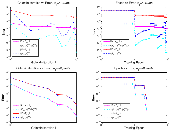
- [Section 6.1.4, Figure 6] For the case omega=64*pi, the caption gives n1=21 for the L2-error panel and n1=13 for the energy-norm panel; please clarify whether this difference is intentional.
- [Section 6.1.1, Figure 1 caption] The label '(Up-Bottom)' appears to be a typo; it likely should read '(Right-Bottom)' or simply '(Bottom)'.
Circularity Check
No circularity: the convergence result is conditional on an explicit quasi-maximization assumption; the main proof gap in Lemma 4.1 is a dropped residual scale, not a circular identification.
full rationale
The claimed results are not circular in the input/output sense. Theorem 4.1 is an implication: if φNN_j satisfies the explicit quasi-maximization inequality (4.19) of Definition 4.1 with δ_j = (2τ_j/(2−τ_j))², then the energy error contracts by the stated factor. The proof uses only Galerkin orthogonality and Lemma 4.1. Lemma 4.1 in turn is conditional on (4.19) and on the plane-wave approximation estimate (3.15) imported from [16, Lemma 4.4] and [23, Corollary 5.5]; these are external, independently published approximation results, not the target theorem. Self-citations ([1], [14]–[16], [34]) supply framework facts such as the norm property of a(·,·) and universal approximation, which are published with independent derivation and are not used to presuppose convergence. No fitted parameter is renamed as a prediction; η(ui−1,φNN_i) is proposed as an equivalent error estimator only under the same conditional inequality. Two caveats prevent a clean endorsement. First, the proof of Lemma 4.1 is not valid as written: from (4.16), ⟨r(u_{i−1}),v⟩ = |||u−u_{i−1}||| Re{a(φ_i,v)}, so (4.19) gives Re{a(φ_i,φNN_i)} ≥ sup_{Vσ∩B} Re{a(φ_i,v)} − δ_i/|||u−u_{i−1}|||, not the −δ_i used in the proof; the derived bound (4.28) therefore needs a relative-tolerance version of (4.19) and is not established. This is an internal proof gap, not circularity. Second, Algorithm 2 gives no guarantee or verification that the training output satisfies (4.19), so the practical claim is conditional. These concerns affect correctness, not whether the derivation reduces to its inputs.
Assumptions & free parameters
free parameters (4)
- Helmholtz DG weights alpha, beta =
alpha = omega^2, beta = 1
- Maxwell DG weights rho1, rho2 =
rho1 = rho2 = 1
- Tolerance parameters tau_i, delta_i =
delta_i = (2 tau_i / (2 - tau_i))^2, tau_i < 0.522
- Training and stopping tolerances =
tol = 1e-6, epsilon = 1e-6 or 1e-8
assumptions (4)
- domain assumption a(.,.) defines a norm on V(Th) for the Helmholtz and Maxwell variational problems
- standard math Plane wave neural networks V^sigma_n are dense in H^s(Th) via Lemma 3.1 from [16,23]
- domain assumption The normalized error phi_i admits a sufficiently regular representation in H^s(Th)
- ad hoc to paper Adam training returns a phi^NN_i satisfying the quasi-maximization inequality (4.19)
Cite this review
Pith. "Pith review of A discontinuous Galerkin plane wave neural network method for Helmholtz equation and Maxwell's equations." pith.science (2026). https://pith.science/paper/GVDL42EX
@misc{pith2026250609309,
  author       = {Pith},
  title        = {Pith review of: A discontinuous Galerkin plane wave neural network method for Helmholtz equation and Maxwell's equations},
  year         = {2026},
  howpublished = {\url{https://pith.science/paper/GVDL42EX}},
  note         = {Machine review of arXiv:2506.09309}
}
abstract
In this paper we propose a discontinuous Galerkin plane wave neural network (DGPWNN) method for approximately solving Helmholtz equation and Maxwell's equations. In this method, we define an elliptic-type variational problem as in the plane wave least square method with $h-$refinement and introduce the adaptive construction of recursively augmented discontinuous Galerkin subspaces whose basis functions are realizations of element-wise neural network functions with $hp-$refinement, where the activation function is chosen as a complex-valued exponential function like the plane wave function. A sequence of basis functions approaching the unit residuals are recursively generated by iteratively solving quasi-maximization problems associated with the underlying residual functionals and the intersection of the closed unit ball and discontinuous plane wave neural network spaces. The convergence results of the DGPWNN method are established without the assumption on the boundedness of the neural network parameters. Numerical experiments confirm the effectiveness of the proposed method.
Figures


Figures from the paper (5 more)


Reference graph
Works this paper leans on
-
[1]
M. Ainsworth and J. Dong, Galerkin neural networks: A framework for approximating varia- tional equations with error control, SIAM J. Sci. Comput., 43(2021), pp. A2474-A2501
work page 2021
- [2]
-
[3]
G. Bao, H. Zhang and J. Zou, Unique determination of periodic polyhedral structures by scat- tered electromagnetic fields, Trans. Amer. Math. Soc., 363 (2011), pp. 4527-4551
work page 2011
-
[4]
J. Berg and K. Nystr ¨om, A unified deep artificial neural network approach to partial differential equations in complex geometries, Neurocomputing, 317 (2018), pp. 28-41
work page 2018
-
[5]
Cybenko, Approximation by superpositions of a sigmoidal function, Math
G. Cybenko, Approximation by superpositions of a sigmoidal function, Math. Control Signals Systems, 2 (1989), pp. 303-314
work page 1989
-
[6]
W. E and B. Yu, The deep Ritz method: A deep learning-based numerical algorithm for solving variational problems, Commun. Math. Stat., 6 (2018), pp. 1-12
work page 2018
-
[7]
Folland, Real Analysis: Modern Techniques and Their Applications, Pure Appl
G. Folland, Real Analysis: Modern Techniques and Their Applications, Pure Appl. Math. (N. Y .) 40, John Wiley & Sons, New York, 1999
work page 1999
-
[8]
C. Gittelson, R. Hiptmair and I. Perugia, Plane wave discontinuous Galerkin methods: Analysis of the h-version, ESAIM Math. Model. Numer. Anal., 43 (2009), pp. 297-331
work page 2009
Show all 37 references
-
[9]
J. He, L. Li, J. Xu, and C. Zheng, ReLU deep neural networks and linear finite elements, J. Comput. Math., 38 (2020), pp. 502-527. 29
2020
-
[10]
Hiptmair, A
R. Hiptmair, A. Moiola, and I. Perugia, Plane wave discontinuous Galerkin methods for the 2D Helmholtz equation: analysis of the p-version. SIAM J. Numer. Anal., 49(2011), pp. 264-284
2011
-
[11]
Hiptmair, A
R. Hiptmair, A. Moiola, and I. Perugia, Error analysis of Trefftz-discontinuous Galerkin methods for the time-harmonic Maxwell equations, Math. Comp., 82(2013), pp. 247-268
2013
-
[12]
Hiptmair, A
R. Hiptmair, A. Moiola and I. Perugia, A survey of Tre fftz methods for the Helmholtz equation. In: Building Bridges: Con- nections and Challenges in Modern Approaches to Numerical Partial Differential Equations, Springer International Publishing, (2015), pp. 237-279
2015
-
[13]
Hornik, Approximation capabilities of multilayer feedforward networks, Neural Netw., 4(1991), pp
K. Hornik, Approximation capabilities of multilayer feedforward networks, Neural Netw., 4(1991), pp. 251-257
1991
-
[14]
Hu and L
Q. Hu and L. Yuan, A weighted variational formulation based on plane wave basis for discretiza- tion of Helmholtz equations, Int. J. Numer. Anal. Model., 11(2014), pp. 587-607
2014
-
[15]
Hu and L
Q. Hu and L. Yuan, A Plane Wave Least-Squares Method for Time-Harmonic Maxwell’s Equa- tions in Absorbing Media, SIAM J. Sci. Comput., 36(2014), pp. A1911-A1936
2014
-
[16]
Hu and L
Q. Hu and L. Yuan, A Plane wave method combined with local spectral elements for nonho- mogeneous Helmholtz equation and time-harmonic Maxwell equations, Adv. Comput. Math., 44(2018), pp. 245-275
2018
-
[17]
Huttunen, P
T. Huttunen, P. Gamallo and R. Astley, Comparison of two wave element methods for the Helmholtz problem, Commun. Numer. Meth. Engng., 25(2009), pp. 35-52
2009
-
[18]
Huttunen, J
T. Huttunen, J. Kaipio and P. Monk. The perfectly matched layer for the ultra weak variational formulation of the 3D Helmholtz equation, Int. J. Numer. Meth. Engng., 61(2004), pp. 1072- 1092
2004
-
[19]
Kharazmi, Z
E. Kharazmi, Z. Zhang, and G. Karniadakis, Variational Physics-Informed Neural Networks for Solving Partial Differential Equations, preprint, https://arxiv.org/abs/1912.00873, 2019
1912 arXiv
-
[20]
Leshno, V
M. Leshno, V . Y . Lin, A. Pinkus, and S. Schocken, Multilayer feedforward networks with a nonpolynomial activation function can approximate any function, Neural Netw., 6 (1993), pp. 861-867
1993
-
[21]
A. Moiola, Tre fftz-discontinuous Galerkin Methods for Time-Harmonic Wave Prob- lems, dissertation, ETH Zurich, Switzerland, 2012; also available online from http://ecollection.library.ethz.ch/view/eth:4515?q=moiola
2012
-
[22]
Moiola and I
A. Moiola and I. Perugia, A space-time Tre fftz discontinuous Galerkin method for the acoustic wave equation in first-order formulation, Numer. Math., 138(2018), pp. 389-435
2018
-
[23]
Moiola, R
A. Moiola, R. Hiptmair, and I. Perugia, Plane wave approximation of homogeneous Helmholtz solutions, Z. Angew. Math. Phys., 62(2011), pp. 809-837
2011
-
[24]
Monk and D
P. Monk and D. Wang, A least-squares method for the helmholtz equation, Comput. Methods Appl. Mech. Engrg., 175(1999), pp. 121-136
1999
-
[25]
Parolin, D
E. Parolin, D. Huybrechs and A. Moiola, Stable approximation of Helmholtz solutions by evanescent plane waves, ESAIM: M2AN, 57(2023), pp. 3499-3536. 30
2023
-
[26]
J. Peng, J. Wang and S. Shu, Adaptive BDDC algorithms for the system arising from plane wave discretization of Helmholtz equations, Int. J. Numer. Methods Eng., 116(2018), pp. 683-707
2018
-
[27]
J. Peng, S. Shu, J. Wang and L. Zhong, Adaptive-Multilevel BDDC algorithm for three- dimensional plane wave Helmholtz systems, J. Comput. Appl. Math., 381(2021), Article ID: 113011
2021
-
[28]
Petersen, M
P. Petersen, M. Raslan, and F. V oigtlaender, Topological properties of the set of functions gener- ated by neural networks of fixed size, Found. Comput. Math., 21 (2021), pp. 375-444
2021
-
[29]
Raissi, P
M. Raissi, P. Perdikaris, and G. Karniadakis, Physics-informed neural networks: A deep learn- ing framework for solving forward and inverse problems involving nonlinear partial differential equations, J. Comput. Phys., 378 (2019), pp. 686-707
2019
-
[30]
Y . Shin, Z. Zhang, G. Karniadakis, Error estimates of residual minimization using neural net- works for linear PDEs, 2020, arXiv:2010.08019
2020 arXiv
-
[31]
Yeung, K
T. Yeung, K. Cheung, E. Chung, S. Fu, J. Qian, Learning rays via deep neural network in a ray-based IPDG method for high-frequency Helmholtz equations in inhomogeneous media, J. Comput. Phys., 465 (2022), 111380
2022
-
[32]
Yuan and Q
L. Yuan and Q. Hu, A PWDG method for the Maxwell system in anisotropic media with piece- wise constant coefficient matrix, ESAIM:M2AN, 58(2024), pp. 1-22
2024
-
[33]
L. Yuan, X. Wang and X. Yue, A space-time Tre fftz dG method for the second order time- dependent Maxwell system in anisotropic media, J. Comput. Math., doi:10.4208 /jcm.2410- m2024-0141, 2024
2024
-
[34]
Yuan and Q
L. Yuan and Q. Hu, A discontinuous plane wave neural network method for Helmholtz equation and time-harmonic Maxwell’s equations, Adv. Comput. Math., 51(2025): 18
2025
-
[35]
Y . Zang, G. Bao, X. Ye, and H. Zhou, Weak adversarial networks for high-dimensional partial differential equations, J. Comput. Phys., 411 (2020), Article ID: 109409
2020
-
[36]
Zhang, C
Y . Zhang, C. Chen, N. Shi, R. Sun and Z. Luo, Adam Can Converge Without Any Modification On Update Rules, Part of Advances in Neural Information Processing Systems 35, (NeurIPS 2022)
2022
-
[37]
M. Zhao, N. Zhu and L. Wang, The electromagnetic scattering from multiple arbitrarily shaped cavities with inhomogeneous anisotropic media, J. Comput. Phys., 489(2023), 112274. 31
2023
Reviewed August 7, 2026 · model on record in the stance chip above.
Discussion (0). Continue with ORCID to comment.