REVIEW 3 major objections 4 minor 16 references
Self-Exciting Multifractional Processes
T0 review · 3 major / 4 minor · reviewed 2026-08-14 · deepseek-v4-flash
Pith's one-line read A stochastic Volterra equation with a state-dependent power kernel is shown to have a unique solution, the self-exciting multifractional process.
desk verdict The SEM construction is new and the main existence/EM results are sound once you fix two typos; the real mathematical gap is the gamma extension's false Lipschitz estimate, not Lemma 4. read the letter →
The pith
A machine-rendered reading of the paper's core claim, the machinery that carries it, and where it could break.
The reading
What carries the argument
The load-bearing machinery is a general existence and uniqueness theorem for stochastic Volterra equations with singular kernels, applied to $\sigma(t,s,x)=(t-s)^{h(t,x)-1/2}$. The theorem requires linear growth and Lipschitz conditions controlled by a Volterra kernel $k\in K_0$; the paper verifies these with $k(t,s)=C_T(t-s)^{2h_*-1}$, after bounding the difference of two power functions by a logarithmic factor. A second bound, Lemma 7, controls the time-increment of the kernel by an integrable factor $\lambda_\gamma(t,t',s)$, and a standard moment-based continuity criterion converts this into Hölder paths. For the Euler--Maruyama error, the paper uses a fractional Gronwall inequality to turn a Volterra integral bound on the mean-square error into the strong rate $|\Delta t|^\gamma$.
What would settle it
Evaluate inequality (3.2) at $t-s=2$ with $h_*=0.1$, $h(t,x)=0.9$, $h(t,y)=0.1$, and $|x-y|=1$: the left side is $(2^{0.4}-2^{-0.4})^2\approx 0.315$, while the right side is $2^{-0.8}(\log 2)^2\approx 0.276$. The inequality fails at this one point, so the kernel does not satisfy the claimed Lipschitz control and the existence proof's load-bearing estimate is false.
Extended reading notes
Core claim
The central claim is that the equation $X_t^h = g(t) + \int_0^t (t-s)^{h(t,X_s^h)-1/2}\,dB_s$, with $h$ a bounded Lipschitz function taking values in $(0,1)$, has a unique solution with finite moments of all orders, and this solution has $\alpha$-Hölder paths for every $\alpha < h_* \wedge \delta$ when $g$ satisfies the paper's continuity condition H4. The paper calls this solution a self-exciting multifractional process (SEM). The printed statement of Theorem 5 writes $h(t,X_t^h)$ in the integrand, but the definition in (1.2), the proof, and all subsequent estimates use $h(t,X_s^h)$; the latter is the operative equation. The same existence and regularity program is carried out for a damped version, the SEM-Gamma process, whose kernel is multiplied by $\exp(-f(t,X_s^h)(t-s))$.
Load-bearing premise
The load-bearing premise is that the kernel's dependence on the current state is controlled by the printed estimate for every time gap; that estimate is too small when the time gap exceeds one, so the existence proof as written depends on an inequality that fails.
Editorial extensions
If this is right
- The discrete self-excited multifractional model now has a rigorously defined continuous-time target, so simulation studies can be run against a well-posed process.
- Because the SEM process has finite moments and Hölder paths with exponent controlled by $h_*$, it can serve as a noise model where the local roughness depends on the recent history of the process.
- The Euler--Maruyama rate $\gamma<2h_*$ gives a concrete rule: when the self-exciting dynamics produce a low lower-Hurst bound, smaller time steps are needed to keep the mean-square error under control.
- The SEM-Gamma version inherits the same existence and convergence results, and its exponential damping produces a mean-reverting process with intermittency, making it a candidate for turbulence or volatility modeling.
Reading between the lines
- The state-Lipschitz estimate in Lemma 4 could be repaired by adding a bounded term that covers lags away from zero; the paper does not provide that correction, but the structure of the proof suggests the convergence rates would not change.
- The rate dependence on $h_*$ suggests a practical diagnostic: estimating $h_*$ from data would directly quantify how finely a SEM model must be sampled for a given error tolerance.
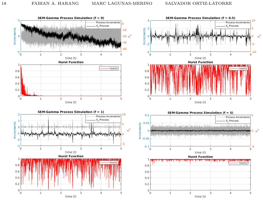
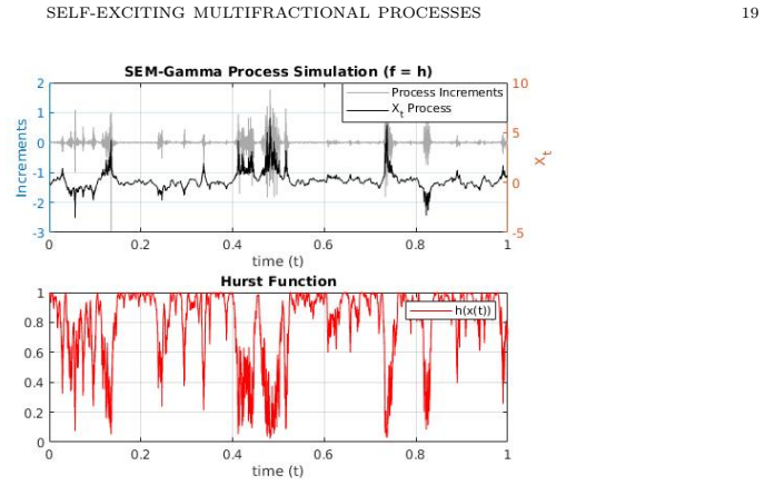
- The reported autocorrelation of absolute increments for SEM-Gamma comes from a single simulation; a systematic Monte Carlo study could test whether this volatility-clustering signal persists across seeds and parameter values.
Signed reviews
Editorial analysis
A structured set of objections, weighed in public.
Referee Report
Summary. The paper introduces a Self-Exciting Multifractional (SEM) process X^h defined as the solution of the Volterra equation X_t = g(t) + ∫_0^t (t-s)^{h(t,X_s)-1/2} dB_s, where h is a time- and path-dependent Hurst function. The authors prove existence and uniqueness via Zhang's theorem (Theorem 5), establish p-th moment bounds, show α-Hölder continuity for α < h_* ∧ δ (Proposition 8), and derive a strong Euler-Maruyama convergence rate |Δt|^γ for any γ < 2h_* (Theorem 9). A damped extension, the SEM-Gamma process, is defined by inserting an exponential factor e^{-f(t,X_s)(t-s)} into the kernel, with analogous existence, regularity, and numerical-scheme results claimed in Section 5. The paper ends with simulations and a discussion of applications to self-exciting phenomena such as earthquakes and financial crashes.
Significance. If the technical issues are repaired, the SEM class is a natural continuous-time counterpart to the Sornette–Filimonov discrete self-excited multifractional model, and the paper gives a serious application of Zhang's stochastic Volterra framework rather than a heuristic construction. The proof strategy is non-circular: existence and moment bounds reduce to external results (Zhang [16], the fractional Gronwall inequality of Ye–Gao–Ding) and standard inequalities, and no data fitting or target-driven construction is involved. The explicit convergence rate 2h_* for the Euler–Maruyama scheme is a useful quantitative feature. However, as written, the SEM-Gamma existence theorem is not proved, and several theorem statements contain errors that must be corrected before the results can be accepted.
major comments (3)
- [Theorem 5, Eq. (3.5) and Section 5, Eq. (5.4)] Equation (3.5) in Theorem 5 writes h(t, X^h_t) inside the integrand, and equation (5.4) writes h(t, X^{h,f}_t) and f(t, X^{h,f}_t). Taken literally, the integrand is not F_s-adapted, and Zhang's Theorem 2 cannot be invoked; the displayed definition is therefore not the process whose existence is proved. The proof, Proposition 8, and the original equations (1.2) and (5.1) use h(t,X_s) (and f(t,X_s)), so the intended statement is clear, but the displayed equations must be corrected before the results can be taken as stated.
- [Lemma 15, Eq. (5.3)] The SEM-Gamma Lipschitz estimate (5.3) is false as printed: for t-s=1 the right-hand side is zero, whereas the left-hand side equals |e^{-f(t,x)}-e^{-f(t,y)}|^2, which is nonzero for, e.g., f(t,x)=1+|x| and x≠y. In the proof, the term |f(t,x)-f(t,y)||t-s| arising from the exponential factor is dropped. Consequently the H2 hypothesis for Zhang's theorem is not verified for the SEM-Gamma kernel, and the existence statement for (5.4) is not proved. A repair is available by taking k2(t,s)=C_T[(t-s)^{2h_*-1}|\log(t-s)|^2+1], which lies in K0, but this corrected kernel is not given in the paper.
- [Section 4.2, Examples] The functions h(x)=1/2 - 1/(2(1+x^2)) and h(x)=1/(1+x^2) take values arbitrarily close to 0, and the first satisfies h(0)=0, so they do not satisfy Definition 3, which requires [h_*,h^*] ⊂ (0,1) with h_*>0. The simulations in Figures 4.2 and 4.3 therefore correspond to a regime not covered by Theorems 5, 8, and 9. Please either restrict the examples to functions with a positive lower bound (e.g., by adding a small ε) or explicitly state that these simulations are outside the theoretical framework.
minor comments (4)
- [Theorem 5] The moment bound in Theorem 5 displays the exponent h_*-1/2 in the integral term; consistency with k1 in Lemma 4 and with Zhang's Theorem 2 requires the exponent 2h_*-1.
- [Lemma 4, proof of (3.2)] In the case |t-s|≥1 the proof bounds the difference by C_T|x-y|^2, but the displayed estimate (3.2) contains an additional |\log(t-s)|^2 factor that vanishes at t-s=1. The conclusion is true—near t-s=1 the left side also vanishes at the rate |\log(t-s)|^2—but the written proof should state this mean-value argument explicitly.
- [Theorem 9, proof of (4.5)] The bound |\log(t-s)|^2 ≤ C (t-s)^{-2δ} is used for all s<t, but it only holds for t-s<1. The contribution from t-s≥1 is harmless and can be handled by splitting the integral; please make this explicit.
- [Various] There are several typographical and reference issues: equation (5.4) repeats the X_t/X_s typo; the text before Lemma 16 says 'Theorem(18)' instead of 'Theorem 18'; reference [13] lacks volume and page details; and the phrase 'h = 1 any time the sample path crossed the x-axis again' is grammatically unclear and should be rewritten.
Circularity Check
No significant circularity: the paper's load-bearing claims are proved from stated assumptions using external existence theorems and standard inequalities.
full rationale
The paper's derivations are self-contained in the relevant sense. The SEM process is defined by a stochastic Volterra equation, and the existence, uniqueness, moment bounds, Hölder regularity, and Euler-Maruyama convergence are all obtained by checking Zhang's hypotheses H1–H2 and then invoking external benchmarks (Zhang's existence theorem [16] and the fractional Gronwall lemma [14]). No parameter is fitted to data, no prediction is a renamed input, and no load-bearing step is justified only by a citation to the present authors. The self-referential appearance of h(t, X_s) inside the integrand is genuine fixed-point structure, not proof-level circularity: Definition 3, Lemma 4, Lemma 7, and Theorem 5 reduce the verification of Zhang's hypotheses to Lipschitz and boundedness assumptions on h, with the target equation's solution as the conclusion rather than as an input. Even the convergence result in Theorem 9 is derived from the already-proved moment estimates rather than assumed. The printed h(t, X^h_t) in Eq. (3.5) and the possible failure of Lemma 15's estimate near lag one are correctness concerns, not instances of circularity. Hence no significant circularity is present.
Assumptions & free parameters
assumptions (6)
- standard math Zhang's existence and uniqueness theorem for stochastic Volterra equations with singular kernels (Theorem 2, reference [16])
- standard math Burkholder-Davis-Gundy inequality
- standard math Kolmogorov's continuity theorem
- standard math Fractional Gronwall inequality (Ye-Gao-Ding, reference [14])
- domain assumption Hurst function h is bounded in (h_*, h^*) ⊂ (0,1) and Lipschitz in time and space
- domain assumption The forcing process g satisfies Zhang's H3 and the regularity H4 (continuity, moment bounds)
Cite this review
Pith. "Pith review of Self-Exciting Multifractional Processes." pith.science (2026). https://pith.science/paper/H4N6NJ52
@misc{pith2026190805523,
  author       = {Pith},
  title        = {Pith review of: Self-Exciting Multifractional Processes},
  year         = {2026},
  howpublished = {\url{https://pith.science/paper/H4N6NJ52}},
  note         = {Machine review of arXiv:1908.05523}
}
read the original abstract
We propose a new multifractional stochastic process which allows for self-exciting behavior, similar to what can be seen for example in earthquakes and other self-organizing phenomena. The process can be seen as an extension of a multifractional Brownian motion, where the Hurst function is dependent on the past of the process. We define this through a stochastic Volterra equation, and we prove existence and uniqueness of this equation, as well as give bounds on the p-order moments, for all p>=1. We show convergence of an Euler-Maruyama scheme for the process, and also give the rate of convergence, which is depending on the self-exciting dynamics of the process. Moreover, we discuss different applications of this process, and give examples of different functions to model self-exciting behavior.
Figures


Figures from the paper (5 more)



Reference graph
Works this paper leans on
-
[16]
Zhang, X. (2010). Stochastic Volterra equations in Banach spaces and stochastic partial differential equation.J. Funct. Anal.258, 1361–1425
work page 2010
-
[1]
Barndorff-Nielsen, O. E. (2016). Gamma kernels andbss/lss processes. InAdvanced modelling in mathematical finance. vol. 189 ofSpringer Proc. Math. Stat.Springer, Cham pp. 41–61
work page 2016
-
[2]
Benassi, A., Jaff ard, S. and Roux, D. (1997). Elliptic Gaussian random processes.Rev. Mat. Iberoamericana 13, 19–90
work page 1997
-
[3]
Bianchi, S., Pantanella, A. and Pianese, A. (2013). Modeling stock prices by multifractional Brownian motion: an improved estimation of the pointwise regularity.Quant. Finance 13, 1317–1330
work page 2013
-
[4]
Bianchi, S., Pantanella, A. and Pianese, A. (2015). Efficient markets and behavioral finance: a comprehensive multifractional model.Adv. Complex Syst.18, 1550001, 29
work page 2015
-
[5]
Bianchi, S. and Pianese, A. (2007). Modelling stock price movements: multifractality or multifractionality? Quant. Finance 7, 301–319. 24 F ABIAN A. HARANG MARC LAGUNAS-MERINO SAL V ADOR ORTIZ-LATORRE
work page 2007
-
[6]
Bianchi, S. and Pianese, A. (2015). Asset price modeling: from fractional to multifractional processes. InFuture perspectives in risk models and finance. vol. 211 ofInternat. Ser. Oper. Res. Management Sci.Springer, Cham pp. 247–285
work page 2015
-
[7]
Cont, R. and Tankov, P. (2004). Financial modelling with jump processes. Chapman & Hall/CRC Financial Mathematics Series. Chapman & Hall/CRC, Boca Raton, FL
work page 2004
Show all 16 references
-
[8]
and Véhel, J
Corlay, S., Lebovits, J. and Véhel, J. L. (2014). Multifractional stochastic volatility models.Math. Finance 24, 364–402
2014
-
[9]
Ha wkes, A. G. (2018). Hawkes processes and their applications to finance: a review.Quant. Finance 18, 193–198
2018
-
[10]
Ioannis Karatzas, S. S. (1998). Brownian motion and stochastic calculus, second edition. Springer
1998
-
[11]
and Véhel, J
Lebovits, J. and Véhel, J. L. (2014). White noise-based stochastic calculus with respect to multifractional Brownian motion.Stochastics 86, 87–124
2014
-
[12]
and Palazzo, A
Pianese, A., Bianchi, S. and Palazzo, A. M. (2018). Fast and unbiased estimator of the time-dependent Hurst exponent. Chaos 28, 031102, 6
2018
-
[13]
and Filimonov, V
Sornette, D. and Filimonov, V. (2011). Self-excited multifractal dynamics.Europhysics Letters Association
2011
-
[14]
and Ding, Y
Ye, H., Gao, J. and Ding, Y. (2007). A generalized Gronwall inequality and its application to a fractional differential equation.J. Math. Anal. Appl.328, 1075–1081
2007
-
[15]
Zhang, X. (2008). Euler schemes and large deviations for stochastic Volterra equations with singular kernels.J. Differential Equations.244, 2226–2250
2008
Reviewed August 14, 2026 · model on record in the stance chip above.
Discussion (0). Continue with ORCID to comment.