REVIEW 3 major objections 4 minor 26 references
Identification of Differential Equations by Dynamics-Guided Weighted Weak Form with Voting
T0 review · 3 major / 4 minor · reviewed 2026-08-07 · deepseek-v4-flash
Pith's one-line read Weighting the weak form of a PDE by per-term dynamics indicators, then voting over several such weightings, identifies both the equation terms and their coefficients from a single noisy trajectory.
desk verdict Solid extension of weak-form PDE discovery with a meaningful new weighting-plus-voting scheme; the empirical case is stronger than the theory, and the missing weighting ablation is the main thing a referee should push on. read the letter →
The pith
A machine-rendered reading of the paper's core claim, the machinery that carries it, and where it could break.
The reading
What carries the argument
The machinery is the dynamics indicator $r(h,\partial_t^{\gamma}\partial_x^{\alpha}u^{\beta})$ of (8)-(9): the $\beta$-scaled absolute value of the weak form of $u^{\beta-1}$ against the differentiated test function. Stacking these indicators for a fixed reference feature gives a diagonal weight matrix $R^{(m)}$, and the linear system $R^{(m)}Wa=R^{(m)}b$ is a preconditioned least-squares problem whose residual is heavier where the dynamics are strong. The second piece is two-stage voting: occurrence voting over the five weight matrices (threshold $\rho=25\%$) removes features that are not repeatedly active, and coefficient voting (threshold $\upsilon=5\%$) removes small average coefficients; the final coefficient recovery rescales each library column by the average leading error coefficient before solving the least-squares problem.
What would settle it
Take one noisy trajectory, build the dynamics weights from the noisy data as the algorithm does, and separately build weights from the underlying noiseless solution of the same trajectory; if the two pipelines identify different equations at the same nominal noise level, the fixed-weight error bound is not describing the algorithm as run, and a second experiment that adds extra noise only inside the high-dynamic regions would make the discrepancy unambiguous.
Extended reading notes
Core claim
The central claim is that a dynamics-guided weighting of localized test functions, followed by occurrence and coefficient voting, identifies the correct differential equation from one trajectory of noisy data. For each reference feature $g_m$, the weight matrix $R^{(m)}$ is diagonal with entries $r(h,g_m)=\beta\,|\int_{\Omega_h} u^{\beta-1}\partial_t^{\gamma}\partial_x^{\alpha}\phi_h\,dxdt|$, the leading coefficient of the noise in a Taylor expansion; the algorithm solves the preconditioned least-squares system $R^{(m)}Wa=R^{(m)}b$ for five reference features, records which coefficients survive, trims low-occurrence and low-magnitude candidates, and computes final coefficients from a rescaled least-squares problem on the surviving support. The error theorem states that the residual at the true coefficient vector is bounded by $O((\Delta x\Delta t)^2)+r_hS_h^*\epsilon+O(r_h\epsilon^2)$, so the weighting concentrates the suppression of noise at the high-dynamic rows, and the same bound shows consistency as the grid and noise go to zero. The discovery is that the data itself can select the informative test-function regions, rather than relying on fixed or random test functions.
Load-bearing premise
The analysis treats the weight matrices as fixed, but the algorithm computes them from the same noisy data that forms the equations, so the bound does not cover the weights actually used; if the weights become correlated with the noise realization, the claimed benefit of weighting could vanish.
Editorial extensions
If this is right
- A single noisy trajectory is enough to recover the equation's support and coefficients at noise levels where the unweighted weak form starts to fail.
- High-dynamic regions are the informative regions: weighting them acts as a preconditioner, so the approach is not tied to a specific library shape and should transfer to larger libraries and higher dimensions.
- Voting across several dynamics-based weightings removes false positives that any single weighting would report.
- The error analysis preserves the stability of the weak form: the residual vanishes as $\Delta x$, $\Delta t$, and $\epsilon$ go to zero, unlike differential-form discretizations whose error can blow up.
- The construction extends to 2D and coupled systems, since the same dynamics indicators are defined per component and per spatial direction.
Reading between the lines
- One consequence the paper leaves implicit is that the dynamics indicators form a data-quality map: large $r(h,g_m)$ marks regions where a small noise in $u$ amplifies into a large weak-form error, so the same indicators could drive adaptive mesh refinement or sensor placement.
- A natural test of the weighting is to compare weights computed from the noisy trajectory with weights computed from the same trajectory's noiseless solution; a large difference in the identified equation would indicate that the data-dependence of the weights needs its own analysis.
- The fixed thresholds $\rho=25\%$ and $\upsilon=5\%$ could be replaced by a stability-selection or bootstrap rule, which would let the method adapt to unknown sparsity instead of using preset values.
- The five reference features are themselves a design choice; the voting record shows how often each feature casts a deciding vote, so one could measure whether a smaller set of reference features suffices.
Editorial analysis
A structured set of objections, weighed in public.
Referee Report
Summary. The paper proposes Ident-WV, a method for identifying differential equations from a single trajectory of noisy observations. The method builds a weak-form linear system from localized test functions, multiplies the system by a diagonal weight matrix constructed from dynamics indicators (Eqs. (8)-(9)), solves a sparse regression problem for each of several reference features, and then applies occurrence voting followed by coefficient voting to select the active features. Coefficients are recovered by a rescaled least-squares solve (Eq. (16)). The authors provide an error analysis in Section 4 bounding the residual at the true coefficient for a fixed weight matrix, and they report extensive numerical comparisons against WeakIdent, WeakSINDy, and Ensemble-SINDy on KdV, heat, transport, Burgers, Kuramoto-Sivashinsky, nonlinear Schrödinger, and porous medium equations.
Significance. If the claims hold, the paper offers a practically useful contribution to PDE discovery from noisy data: it combines the robustness of weak formulations with data-adaptive weighting and a voting mechanism, and the experiments are considerably broader than those in several prior weak-form works. The numerical evidence is extensive and includes a comparison with an ensemble method, which is commendable. The proposed voting strategy is simple and sensible, and the fixed-weight residual bound in Theorem 1 is valid as far as it goes. However, the significance is tempered by two gaps: the theoretical analysis does not cover the data-dependent weights actually used in the algorithm, and the experiments do not isolate the weighting step from the voting step. These issues leave the central novelty of the paper under-supported.
major comments (3)
- [Section 4, Theorem 1] Theorem 1 bounds the residual at the true coefficient a* for a fixed weight matrix R, but the algorithm computes R(m) from the same noisy data D used to form W and b (Eqs. (8)-(9)). The bound |(e_{a*})_h| ≤ O((ΔxΔt)^2) + r_h S*_h ε + O(r_h ε^2) omits the coupling terms δR·E(0) and δR·δE that arise because r_h depends on the noise realization. Moreover, the text asserts that sparse recovery follows if R(m)W satisfies the incoherence property or RIP, but no such condition is verified and the paper does not connect the residual bound to support or coefficient recovery. Please either extend the analysis to the data-dependent weight case, or explicitly state that Theorem 1 applies only to an idealized fixed-weight version and add numerical evidence (e.g., oracle weights or a convergence-in-r study) to justify the weighting step used in practice.
- [Section 5 (all subsections)] No experiment isolates the contribution of the dynamics-guided weighting. The paper compares Ident-WV to WeakIdent, WeakSINDy, and Ensemble-SINDy, but never runs Ident-WV with R = I (unweighted) or with oracle weights computed from the noiseless solution. Since the title and abstract emphasize the weighted weak form as the key contribution, the observed robustness could in principle be due entirely to the occurrence/coefficient voting. Please add an ablation study that separates the weighting step from the voting step; this is essential to support the paper's central claim.
- [Section 3.4 and Algorithm 1] The occurrence threshold is specified inconsistently: Section 3.4 states 'The threshold ρ = 20% and ν = 5%', while Algorithm 1 gives 'Parameters ρ = 25% and υ = 5%'. Because ρ directly controls which features survive the first voting step, this inconsistency prevents reproduction of the experimental results. Please state the exact threshold used in all experiments, unify the notation (ν vs υ), and report sensitivity of the results to ρ.
minor comments (4)
- [Algorithm 1] There is a typo in Step 8: 'First V oting' should read 'First Voting'.
- [Section 2 vs Section 4] The problem setup assumes i.i.d. Gaussian noise, while Theorem 1 assumes bounded noise with |ε_i^k| ≤ ε. Please clarify the connection (e.g., by stating that the theorem applies to truncated Gaussian noise or that the bound can be extended to sub-Gaussian noise with high probability).
- [Figure 2 caption] The caption says '(b) - (e) display the dynamics indicators R[u2], R[(u2)x], R[(u2)xx], R[(u2)t] when the reference feature is u2, u2x, u2xx, u2t respectively,' but the y-axis labels and text use inconsistent notation (u2 vs u^2). Please standardize the notation.
- [Appendix B] The claim that 'the major improvement in E-SINDy is achieved through library bagging' is based on Figures 15 and 16, but the figures do not explicitly mark which configuration is which beyond the panel labels; adding a short summary of the ranking would help readability.
Circularity Check
No significant circularity: the dynamics-guided weights are data-derived preconditioners, not fitted outputs, and the recovery is validated on synthetic ground-truth equations.
full rationale
The central derivation is self-contained with respect to the input data and the target equation. The dynamics indicators in Eq. (8) and weight matrices in Eq. (9) are computed from the observed data, but they are not fitted to the unknown coefficient vector a, nor is any recovered quantity stated as a prediction that was used to define the weights. The weighted weak form Eq. (10) is a preconditioned linear system whose solution is the coefficient vector; this is a standard estimation procedure, not a self-definitional construction. Theorem 1 bounds the residual at the true coefficient and is a consistency statement about the weighted residual, not a circular derivation of the estimator. The only limitation is that Theorem 1 treats the weights R(m) as fixed even though they depend on the same noisy data; that is a gap between analysis and algorithm, but it does not make the identification circular. The method is validated against WeakIdent, WeakSINDy, and Ensemble-SINDy on synthetic equations with known ground truth, and no parameter fitted to the output is relabeled as a prediction. Citations to WeakIdent [24] by overlapping authors are used for a subroutine and for the high-dynamic-region idea, but the central weighting-and-voting mechanism is proposed and tested in this paper rather than imported as an unverified premise. No circular step can be exhibited from the paper's own equations, so the appropriate finding is no significant circularity.
Assumptions & free parameters
free parameters (4)
- Occurrence threshold rho =
25% (Algorithm 1); 20% (Section 3.4)
- Coefficient threshold upsilon =
5%
- Reference feature set =
{u, u2, (u2)x, (u2)xx, (u2)t}
- Test function count and support =
not specified in the paper
assumptions (5)
- domain assumption The governing PDE is a linear combination of library terms d_x^a u^b (Eq. 3-4).
- standard math Test functions and their derivatives up to the needed order vanish on the boundary of their support.
- domain assumption Noise is i.i.d., zero-mean, bounded, and small enough that the first-order Taylor expansion in Eq. (8) is accurate.
- standard math Trapezoidal rule integration is second-order accurate and the integrands have bounded second derivatives.
- domain assumption WeakIdent sparse recovery on each weighted system produces supports that overlap with the true support often enough for voting to work.
invented entities (1)
-
Dynamics indicator r(h, d_t^gamma d_x^alpha u^beta)
Cite this review
Pith. "Pith review of Identification of Differential Equations by Dynamics-Guided Weighted Weak Form with Voting." pith.science (2026). https://pith.science/paper/HFTBQNAT
@misc{pith2026250603899,
  author       = {Pith},
  title        = {Pith review of: Identification of Differential Equations by Dynamics-Guided Weighted Weak Form with Voting},
  year         = {2026},
  howpublished = {\url{https://pith.science/paper/HFTBQNAT}},
  note         = {Machine review of arXiv:2506.03899}
}
read the original abstract
In the identification of differential equations from data, significant progresses have been made with the weak/integral formulation. In this paper, we explore the direction of finding more efficient and robust test functions adaptively given the observed data. While this is a difficult task, we propose weighting a collection of localized test functions for better identification of differential equations from a single trajectory of noisy observations on the differential equation. We find that using high dynamic regions is effective in finding the equation as well as the coefficients, and propose a dynamics indicator per differential term and weight the weak form accordingly. For stable identification against noise, we further introduce a voting strategy to identify the active features from an ensemble of recovered results by selecting the features that frequently occur in different weighting of test functions. Systematic numerical experiments are provided to demonstrate the robustness of our method.
Figures


Figures from the paper (13 more)




Reference graph
Works this paper leans on
-
[1]
Fitting ordinary differential equations to chaotic data
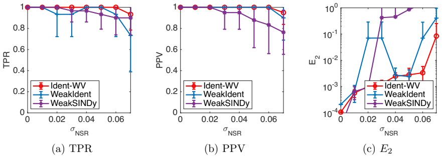
Ellen Baake, Michael Baake, HG Bock, and KM Briggs. Fitting ordinary differential equations to chaotic data. Physical Review A , 45(8):5524, 1992. 17 0 0.02 0.04 0.06<NSR 0 0.2 0.4 0.6 0.8 1TPR Ident-WVWeakIdentWeakSINDy 0 0.02 0.04 0.06<NSR 0 0.2 0.4 0.6 0.8 1PPV Ident-WVWeakIdentWeakSINDy 0 0.02 0.04 0.06<NSR 10-4 10-3 10-2 10-1 100 E2 Ident-WVWeakIdent...
work page 1992
-
[2]
Fitting partial differential equations to space- time dynamics
Markus B¨ ar, Rainer Hegger, and Holger Kantz. Fitting partial differential equations to space- time dynamics. Physical Review E , 59(1):337, 1999
work page 1999
-
[3]
Recent advances in parameter identification techniques for ode
Hans Georg Bock. Recent advances in parameter identification techniques for ode. Numerical treatment of inverse problems in differential and integral equations , pages 95–121, 1983
work page 1983
-
[4]
Automated reverse engineering of nonlinear dynamical systems
Josh Bongard and Hod Lipson. Automated reverse engineering of nonlinear dynamical systems. Proceedings of the National Academy of Sciences , 104(24):9943–9948, 2007
2007
-
[5]
Discovering governing equations from data by sparse identification of nonlinear dynamical systems
Steven L Brunton, Joshua L Proctor, and J Nathan Kutz. Discovering governing equations from data by sparse identification of nonlinear dynamical systems. Proceedings of the National Academy of Sciences, 113(15):3932–3937, 2016
work page 2016
-
[6]
Decoding by linear programming
Emmanuel J Candes and Terence Tao. Decoding by linear programming. IEEE transactions on information theory , 51(12):4203–4215, 2005. 18 0 0.5 1 1.5 <NSR 0 0.2 0.4 0.6 0.8 1 TPR Ident-WV WeakIdent WeakSINDy E-SINDy-DB-5 (a) TPR 0 0.5 1 1.5 <NSR 0 0.2 0.4 0.6 0.8 1 PPV Ident-WV WeakIdent WeakSINDy E-SINDy-DB-5 (b) PPV 0 0.5 1 1.5 <NSR 10-4 10-2 100 E2 Ident...
work page 2005
-
[7]
Uncertainty principles and ideal atomic decomposition
David L Donoho, Xiaoming Huo, et al. Uncertainty principles and ideal atomic decomposition. IEEE transactions on information theory , 47(7):2845–2862, 2001
work page 2001
-
[8]
Urban Fasel, J Nathan Kutz, Bingni W Brunton, and Steven L Brunton. Ensemble-sindy: Robust sparse model discovery in the low-data, high-noise limit, with active learning and control. Proceedings of the Royal Society A , 478(2260):20210904, 2022
work page 2022
Show all 26 references
-
[9]
Robust and optimal sparse regression for nonlinear pde models
Daniel R Gurevich, Patrick AK Reinbold, and Roman O Grigoriev. Robust and optimal sparse regression for nonlinear pde models. Chaos: An Interdisciplinary Journal of Nonlinear Science , 29(10):103113, 2019
2019
-
[10]
Group projected subspace pursuit for block sparse signal reconstruction: Convergence analysis and applications
Roy Y He, Haixia Liu, and Hao Liu. Group projected subspace pursuit for block sparse signal reconstruction: Convergence analysis and applications. Applied and Computational Harmonic Analysis, 75:101726, 2025
2025
-
[11]
Numerical identification of nonlocal potential in aggregation
Yuchen He, Sung Ha Kang, Wenjing Liao, Hao Liu, and Yingjie Liu. Numerical identification of nonlocal potential in aggregation. Communications in Computational Physics , 2022
2022
-
[12]
Robust identification of differential equations by numerical techniques from a single set of noisy observation
Yuchen He, Sung-Ha Kang, Wenjing Liao, Hao Liu, and Yingjie Liu. Robust identification of differential equations by numerical techniques from a single set of noisy observation. SIAM Journal on Scientific Computing , 44(3):A1145–A1175, 2022
2022
-
[13]
Group projected subspace pursuit for identification of variable coefficient differential equations (gp-ident)
Yuchen He, Sung Ha Kang, Wenjing Liao, Hao Liu, and Yingjie Liu. Group projected subspace pursuit for identification of variable coefficient differential equations (gp-ident). Journal of Computational Physics , 494:112526, 2023
2023
-
[14]
How much can one learn a partial differential equation from its solution? Foundations of Computational Mathematics , 24(5):1595–1641, 2024
Yuchen He, Hongkai Zhao, and Yimin Zhong. How much can one learn a partial differential equation from its solution? Foundations of Computational Mathematics , 24(5):1595–1641, 2024
2024
-
[15]
Ident: Identifying differential equations with numerical time evolution
Sung Ha Kang, Wenjing Liao, and Yingjie Liu. Ident: Identifying differential equations with numerical time evolution. Journal of Scientific Computing , 87(1):1–27, 2021. 19
2021
-
[16]
System identification
Lennart Ljung. System identification. Springer, 1998
1998
-
[17]
Weak sindy for partial differential equations
Daniel A Messenger and David M Bortz. Weak sindy for partial differential equations. Journal of Computational Physics , page 110525, 2021
2021
-
[18]
Weak sindy: Galerkin-based data-driven model selection
Daniel A Messenger and David M Bortz. Weak sindy: Galerkin-based data-driven model selection. Multiscale Modeling & Simulation , 19(3):1474–1497, 2021
2021
-
[19]
Parameter identification techniques for partial differential equations
Thomas G M¨ uller and Jens Timmer. Parameter identification techniques for partial differential equations. International Journal of Bifurcation and Chaos , 14(06):2053–2060, 2004
2004
-
[20]
Using noisy or incomplete data to discover models of spatiotemporal dynamics
Patrick AK Reinbold, Daniel R Gurevich, and Roman O Grigoriev. Using noisy or incomplete data to discover models of spatiotemporal dynamics. Physical Review E, 101(1):010203, 2020
2020
-
[21]
Learning partial differential equations via data discovery and sparse opti- mization
Hayden Schaeffer. Learning partial differential equations via data discovery and sparse opti- mization. Proceedings of the Royal Society A: Mathematical, Physical and Engineering Sci- ences, 473(2197):20160446, 2017
2017
-
[22]
Distilling free-form natural laws from experimental data
Michael Schmidt and Hod Lipson. Distilling free-form natural laws from experimental data. Science, 324(5923):81–85, 2009
2009
-
[23]
He, and Hao Liu
Cheng Tang, Roy Y. He, and Hao Liu. Wg-ident: Weak group identification of pdes with varying coefficients, 2025
2025
-
[24]
Weakident: Weak formulation for identifying differential equation using narrow-fit and trimming
Mengyi Tang, Wenjing Liao, Rachel Kuske, and Sung Ha Kang. Weakident: Weak formulation for identifying differential equation using narrow-fit and trimming. Journal of Computational Physics, 483:112069, 2023
2023
-
[25]
Fourier features for identifying differential equations (fourierident)
Mengyi Tang, Hao Liu, Wenjing Liao, and Sung Ha Kang. Fourier features for identifying differential equations (fourierident). arXiv preprint arXiv:2311.16608 , 2023
2023 arXiv
-
[26]
Numerical aspects for approximating governing equations using data
Kailiang Wu and Dongbin Xiu. Numerical aspects for approximating governing equations using data. Journal of Computational Physics , 384:200–221, 2019. A Full results in Section 5.2 In this section, we demonstrate the full results about 1D equations in Table 1 in Section 5.2 wh...
2019
Reviewed August 7, 2026 · model on record in the stance chip above.
Discussion (0). Sign in to comment.