REVIEW 5 major objections 6 minor 35 references
Where are all the dark galaxies? Predicting galaxy/halo locations from their bright neighbors
T0 review · 5 major / 6 minor · reviewed 2026-08-06 · deepseek-v4-flash
Pith's one-line read The paper shows that dark galaxies and dark matter halos can be located from the distances to their two nearest bright neighbors.
desk verdict Interesting empirical fit to dark-object density from bright-neighbor distances, but the predictive claim is undermined by in-sample evaluation and an undefined baseline. read the letter →
The pith
A machine-rendered reading of the paper's core claim, the machinery that carries it, and where it could break.
The reading
What carries the argument
The load-bearing object is the conditional probability density $p(r_1,r_2,r_{12})$, defined in Eq. (3), where $r_1$ and $r_2$ are the distances from a candidate dark object to its first and second nearest bright neighbors and $r_{12}$ is the separation between those two neighbors. The paper models this density with symbolic regression—a machine learning method that searches over closed-form expressions—using a Poisson maximum-likelihood loss (Eq. 12) and a Poisson Information Criterion to select a parsimonious formula. The selected formula, Eq. (15), is the paper's central identity: it expresses the dark-object density as an exponential of a ratio built from the three distances, with mass-dependent dimensionless parameters.
What would settle it
Estimate the same p(r1,r2,r12) from an independent simulation with different resolution or from a complete observational galaxy sample with known completeness, and compare the dark-object density predicted by Eq. (15) with the measured one; if the residuals correlate significantly with large-scale density or tidal shear, the assumption that nearest-neighbor distances suffice is falsified.
Extended reading notes
Core claim
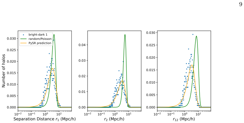
The central claim is that the conditional probability density $p(r_1,r_2,r_{12})$ of a dark object given its two closest bright neighbors is captured by Eq. (15), an exponential function of the rescaled dimensionless distances $\tilde{r}=r\,\bar{n}^{1/3}$: $p=\exp\!\left(\frac{1}{a\tilde{r}_2+b}\left(\frac{c}{2\tilde{r}_2+\tilde{r}_{12}}\right)^{d\tilde{r}_1}+e\right)$, with fitted constants $a,b,c,d,e$ given in Table I for each tracer combination. The same expression, with different parameters, fits the simulated density of dark halos around bright halos, faint galaxies around bright galaxies, and halos around bright galaxies. The paper interprets this as evidence that local gravitational clustering encodes the information needed to locate dark, faint, or otherwise undetectable objects, and shows that maps reconstructed this way correlate with the true dark-object map more strongly than the linear bias prediction at small scales.
Load-bearing premise
The model assumes that once the two distances to the nearest bright neighbors and the distance between them are fixed, the probability of a dark object is fully determined; if other environmental variables (large-scale density, tidal shear, or formation history) also matter, the fitted formula will not generalize to other simulations or to the real sky.
Editorial extensions
If this is right
- Telescope surveys can be pointed at predicted high-probability regions around bright galaxies, increasing the chance of detecting faint dwarf and satellite galaxies.
- Dark sirens—compact-object mergers without electromagnetic counterparts—can be localized better by weighting their sky positions with the predicted halo map, which the paper suggests could sharpen Hubble-constant measurements.
- The same bright-galaxy sample can be used to infer host halo centers, which then predicts where other halos sit, informing weak-lensing searches for dark structure.
- The formula's parameters are specific to tracer type but its form is stable across Illustris-2 and TNG-100, so it may serve as an empirical, simulation-calibrated replacement for scale-dependent bias at quasi-linear scales.
- Future work could extend the k=2 nearest-neighbor statistic to higher k, potentially capturing even more environmental information.
Reading between the lines
- Editorial inference: if Eq. (15) holds for real surveys, it would provide a testable, non-parametric check on ΛCDM structure formation, since the fitted parameters could be compared between simulation and observation without assuming a halo model.
- Editorial inference: because the paper never tests whether adding large-scale density or tidal anisotropy improves the fit, a natural extension is to feed those features to the same regression and see whether the nearest-neighbor variables remain sufficient; this would identify what environmental information is truly encoded.
- Editorial inference: the approach may extend beyond galaxies and halos to any tracers of the same underlying density field, such as X-ray clusters, quasars, or cosmic voids, as long as a 'bright' reference population and a 'dark' target population share clustering physics.
- Editorial inference: the k=2 limitation is imposed by the simplicity of the chosen geometry; allowing k>2 neighbors, or including neighbor luminosities, could break degeneracies in Eq. (15) and might be required when applying the formula to observational data with incompleteness.
Editorial analysis
A structured set of objections, weighed in public.
Referee Report
Summary. The paper uses the PySR symbolic regression package on Illustris-TNG simulations to fit an analytic expression, Eq. (15), for the probability density of finding a 'dark' object (halo or faint galaxy) as a function of the distances to its two nearest 'bright' neighbors and the separation between those neighbors. The authors report that this expression predicts the dark-object number-density map significantly better than a 'linear scale-dependent biasing prediction' at k ~ 1 h/Mpc, and they demonstrate the same functional form across halo-halo, galaxy-galaxy, and halo-galaxy cases, including a cross-check with TNG-100.
Significance. If the predictive claim were properly validated, the paper would provide an interpretable, low-cost mapping from bright galaxy catalogues to dark-matter and faint-galaxy density fields, with potential applications to missing-satellite searches, dark-siren localization, and weak-lensing mass maps. The use of symbolic regression to produce a closed-form expression is a genuine strength: it is human-readable, reproducible, and may transfer across simulations. However, the present evidence does not yet support the core claim of predictive superiority over the stated baseline.
major comments (5)
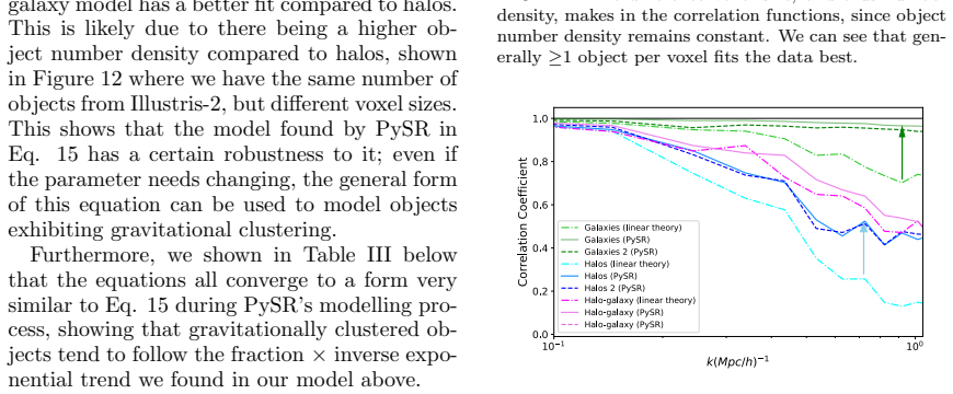
- [Section III, Fig. 9] The correlation coefficients in Fig. 9 are computed on the same Illustris-2 volume used to fit the parameters a, b, c, d, e of Eq. (15) in Table I. This is an in-sample measure of goodness of fit, not a predictive test. The abstract's claim that Eq. (15) can 'predict' dark-object density is therefore not supported by this figure. The authors should provide a train/test split (e.g., fit on one half of the box and test on the other half, or use cross-validation) and report the test-set correlations.
- [Fig. 9 and abstract] The baseline labeled 'linear' in Figs. 9, 11, and 12 is never defined in the text. The abstract calls it a 'linear scale-dependent biasing prediction', but the caption of Fig. 9 refers to 'bright/visible object raw number counts'. No equation, bias parameter, or power-spectrum construction is given. The comparison is not meaningful unless the baseline is specified precisely (for instance, a linear bias model b(k) times the bright-galaxy overdensity, or a linear regression of dark counts on bright counts) and the correlation coefficients are computed for that model.
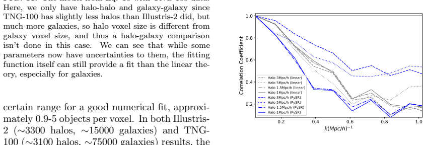
- [Section III, Fig. 11 and Table II] The TNG-100 check is presented as independent support, but Table II shows that all five parameters are refitted on TNG-100. This tests only whether the functional form of Eq. (15) is flexible enough to fit a second simulation; it does not test the predictive power of the parameters derived from Illustris-2. A more informative test would be to apply the Illustris-2 parameters to TNG-100 without refitting, or to fit on TNG-100 and test on Illustris-2, and report the resulting correlations.
- [Fig. 9, Fig. 10, Fig. 12] The correlation coefficients in Figs. 9 and 11 have no error bars, and the significance of the difference between the PySR model and the linear baseline is not quantified. Since Fig. 12 shows that the results depend strongly on voxel size, bootstrap or jackknife uncertainties over the 3D density field should be provided before claiming 'significantly better' performance.
- [Section II.A, Eq. (3)] The model assumes that the conditional probability density of a dark object is fully determined by (r1, r2, r12). This assumption is stated but never tested against alternative environmental variables such as large-scale density, tidal anisotropy, or assembly history. The random-forest importance test in Fig. 5 compares the three distances only to random numbers, not to other physical covariates, so it does not validate the completeness of the chosen descriptor set. If the fitted expression is intended as a predictive tool for real surveys, this missing test weakens the claim of generality.
minor comments (6)
- [Eq. (12)] In Eq. (12), the softening parameter epsilon appears inside the logarithm, so it has a small numerical effect even though the authors state it 'has no effect'; please rephrase to 'negligible effect'.
- [Section II.A] The text says the number of halos in each distance bin is divided by the total number of halos 'to obtain the probability.' Eq. (3) defines a probability density. Please clarify the normalization (per bin width in r1, r2, r12) and state whether the plotted quantities are densities or probabilities.
- [Table I] The fitted parameters in Table I are given without uncertainties. Given the small number of bins and the Poisson noise, reporting uncertainties would help the reader assess the stability of the fit.
- [Fig. 10] The Heaviside threshold applied to the predicted number densities (≤1 object per voxel) is not described in the Methods. Its effect on the correlation coefficients in Fig. 9 should be documented or justified.
- [Figs. 9 and 11] The baseline is called 'linear' in Fig. 9 and 'linear theory' in Fig. 11; please use consistent terminology and explicitly define the model in both captions.
- [Section III, text before Fig. 6] The sentence 'We use the subhalo galaxies as our training set and host halos as our testing set' is unclear, since the subsequent figures show halo-halo and galaxy-galaxy fits without an explicit train/test split; please clarify the intended meaning.
Circularity Check
The headline 'prediction' is an in-sample fit: Eq. 15 is trained on the same Illustris-2 dark-object counts used to compute the Fig. 9 correlations, so the claimed improvement is not an out-of-sample test.
-
fitted input called prediction
[Section III, Eq. 15 and Fig. 9; fitting set up in Section II.C, Eq. 12]
"To calculate the probability of finding a halo or galaxy object in a certain volume element, we model simulation data points by using symbolic regression and the Poisson error function in Eq. 12 as the loss function to be minimized. ... The correlation coefficients between the true 3D dark halo/galaxy map and our machine learning model based on 3D bright objects."
The five parameters of Eq. 15 are fit to Illustris-2 dark-object counts (Section II.C maximizes the Poisson likelihood against per-voxel counts; Table I obtains a-e with curve_fit), and Fig. 9 then correlates the resulting dark-object map with those same true dark-object counts from the same simulation volume. No held-out split separating the fitted dark-object counts from the correlated counts is described for the Illustris-2 curves. The 'prediction' of dark-object density is therefore the fitted density of the training data; its correlation coefficient is an in-sample goodness-of-fit measure, not a predictive test. The abstract's 'significantly better' claim compares this in-sample fit to a raw bright-count map, so the advertised predictive improvement reduces to the fit by construction.
full rationale
The derivation of Eq. 15 is an ordinary symbolic-regression fit: PySR minimizes the Poisson loss (Eq. 12) against Illustris-2 voxel counts and Table I parameters are found by curve_fit. The paper calls this a prediction, but the Fig. 9 correlations use the same Illustris-2 data used for the fit, so the central quantitative claim is a training-set correlation rather than an out-of-sample prediction. The TNG-100 appendix provides some independent grounding, but it refits the five parameters on TNG-100 before evaluating, so it validates the functional form's robustness rather than the predictive power of fixed Table I parameters. A separate correctness issue, not itself circularity: the 'linear' baseline in Fig. 9 is the raw bright-object number-count map, not the 'linear scale-dependent biasing prediction' invoked in the abstract. No load-bearing self-citation or imported uniqueness theorem is present. Because the main claim partially reduces to an in-sample fit, score 6.
Assumptions & free parameters
free parameters (8)
- a =
0.28 (halo-galaxy), 10.0 (halo-halo), 180 (galaxy-galaxy)
- b =
0.057 (halo-galaxy), 28.0 (halo-halo), 210 (galaxy-galaxy)
- c =
0.1 (halo-galaxy), 0.5 (halo-halo), 1.0 (galaxy-galaxy)
- d =
0.1 (halo-galaxy), 2.7 (halo-halo), 8.0 (galaxy-galaxy)
- e =
0.01 (halo-galaxy), 1.7 (halo-halo), 0.7 (galaxy-galaxy)
- Bright/dark mass thresholds =
halo bright >= 1e12 Msun; galaxy bright >= 1e10 Msun; galaxy dark 2e9 to 1e10 Msun
- Voxel size =
3 Mpc/h (default; 1 to 5 Mpc/h tested)
- Heaviside density threshold =
Predictions <= 1 object per voxel set to zero
assumptions (4)
- domain assumption Illustris-TNG simulations faithfully represent the spatial distribution of dark matter halos and galaxies in the real universe.
- domain assumption The probability density of dark objects depends only on r1, r2, and r12 (the nearest two bright neighbors and their separation).
- domain assumption One-to-one baryon mass-luminosity dependence for galaxies and an unknown mass-luminosity dependence for halos.
- standard math Poisson statistics for counts in voxels and Bayes theorem for the null distribution.
Cite this review
Pith. "Pith review of Where are all the dark galaxies? Predicting galaxy/halo locations from their bright neighbors." pith.science (2026). https://pith.science/paper/HHVPU2CB
@misc{pith2026250701814,
  author       = {Pith},
  title        = {Pith review of: Where are all the dark galaxies? Predicting galaxy/halo locations from their bright neighbors},
  year         = {2026},
  howpublished = {\url{https://pith.science/paper/HHVPU2CB}},
  note         = {Machine review of arXiv:2507.01814}
}
abstract
Astronomical objects in our universe that are too faint to be directly detectable exist and are important - an obvious example being dark matter. The same can also apply to very faint baryonic objects, such as low luminosity dwarf galaxies and gravitationally compact objects (e.g., rogue planets, white dwarfs, neutron stars, black holes, dark sirens). While they are very difficult to observe directly, they have locations that are highly important when studying astrophysical phenomena. Here, we use a machine learning algorithm known as symbolic regression to model the probability of a dark object's existence as a function of their separation distances to their closest two ``bright" (directly observable) neighbors, and the distances of these bright objects to each other. An advantage of this algorithm is that it is interpretable by humans and can be used to make reproducible predictions. Galaxies with masses above $10^9 M_{\odot}$ and halos above $10^{12} M_{\odot} $ are the objects that we separate into ``bright" and ``dark" to be used in our analysis. We find that it is possible to predict the density of dark objects using an analytic expression that depends on their distances to their closest bright neighbors in Illustris-TNG galaxy formation simulations, which is significantly better than the (linear) scale-dependent biasing prediction for $k \sim 1.0~ h$Mpc$^{-1}$ (and potentially beyond, if allowed by the resolution). This could potentially open the avenue for finding dark objects based on their vicinity to directly observable bright sources and make future surveys more targeted and efficient.
Figures


Figures from the paper (10 more)




Reference graph
Works this paper leans on
-
[1]
P. A. R. Ade et al. Planck 2015 results. XIII. Cosmological parameters. Astron. Astrophys., 594:A13, 2016
2015
-
[2]
= xi, just like MSE (Eq. 9). Although the number of galaxies/haloes per voxel is xi ≥ 0, the PySR algorithm fit for λ is not necessarily ≥ 0 for every voxel. To ensure that this does not become a problem for the ln function, we can make a change of the variable λ → eϕ, where we fit for ϕ instead. The loss function then becomes ˜L → nX i=1 " eϕ(ri 1,ri 2,ri
-
[3]
− xi 1 − ln eϕ(ri 1,ri 2,ri 12) xi + ϵ # , (12) where ϵ is a softening length to avoid an unde- fined 0 ln |0| in the code (we set ϵ to be 10 −10), although it has no effect on ˜L. The list of equations (also known as the “Pareto front”) that PySR has given us is shown in Table III in the Appendix. Not all separa- tion distances, r1, r2, r12 are used in t...
-
[4]
Marika Asgari, Alexander J. Mead, and Catherine Heymans. The halo model for cos- mology: a pedagogical review. 3 2023
work page 2023
-
[5]
The NANOGrav 15 yr Data Set: Evidence for a Gravitational-wave Background
Gabriella Agazie et al. The NANOGrav 15 yr Data Set: Evidence for a Gravitational-wave Background. Astrophys. J. Lett., 951(1):L8, 2023
work page 2023
-
[6]
Raul E. Angulo and Oliver Hahn. Large-scale dark matter simulations. 12 2021
work page 2021
-
[7]
Asantha Cooray and Ravi K. Sheth. Halo Models of Large Scale Structure. Phys. Rept., 372:1–129, 2002
work page 2002
-
[8]
Nearest neigh- bour distributions: New statistical measures for cosmological clustering
Arka Banerjee and Tom Abel. Nearest neigh- bour distributions: New statistical measures for cosmological clustering. Mon. Not. Roy. Astron. Soc., 500(4):5479–5499, 2020
work page 2020
Show all 35 references
-
[9]
James S. Bullock. Notes on the missing satel- lites problem, 2010
2010
-
[10]
Cosmology with LIGO/Virgo dark sirens: Hubble parameter and modified gravitational wave propagation
Andreas Finke, Stefano Foffa, Francesco Iacov- elli, Michele Maggiore, and Michele Mancar- ella. Cosmology with LIGO/Virgo dark sirens: Hubble parameter and modified gravitational wave propagation. JCAP, 08:026, 2021
2021
-
[11]
Interpretable Machine Learning for Science with PySR and Sym- bolicRegression.jl
Miles Cranmer. Interpretable Machine Learning for Science with PySR and Sym- bolicRegression.jl. arXiv e-prints , page arXiv:2305.01582, May 2023
2023 arXiv
-
[12]
− xi 1 − ln λ(ri 1, ri 2, ri 12) xi # . (11) 6 500 1000 0.00 0.01 0.02 0.03 0.04 ML r1 data r1 analytic r1 500 1000 1500 0.000 0.005 0.010 0.015 0.020 0.025 0.030 0.035 ML r2 data r2 analytic r2 0 500 1000 1500 2000 0.00 0.01 0.02 0.03 0.04 ML r3 data r3 analytic r3 FIG. 3. Ra...
2000
-
[13]
Discovering Symbolic Models from Deep Learning with Inductive Bi- ases
Miles Cranmer, Alvaro Sanchez-Gonzalez, Pe- ter Battaglia, Rui Xu, Kyle Cranmer, David Spergel, and Shirley Ho. Discovering Symbolic Models from Deep Learning with Inductive Bi- ases. 6 2020
2020
-
[14]
Understanding predictive information criteria for Bayesian models
Andrew Gelman, Jessica Hwang, and Aki Ve- htari. Understanding predictive information criteria for Bayesian models. arXiv e-prints, page arXiv:1307.5928, July 2013
2013 arXiv
-
[15]
Harris, K
Charles R. Harris, K. Jarrod Millman, St´ efan J. van der Walt, Ralf Gommers, Pauli Virta- nen, David Cournapeau, Eric Wieser, Ju- lian Taylor, Sebastian Berg, Nathaniel J. Smith, Robert Kern, Matti Picus, Stephan Hoyer, Marten H. van Kerkwijk, Matthew Brett, Allan Haldane, Ja...
2020
-
[16]
Final results of the search for new Milky Way satellites in the Hy- per Suprime-Cam Subaru Strategic Program survey: Discovery of two more candidates
Daisuke Homma et al. Final results of the search for new Milky Way satellites in the Hy- per Suprime-Cam Subaru Strategic Program survey: Discovery of two more candidates. Publ. Astron. Soc. Jap. , 76(4):733–752–752, 2024
2024
-
[17]
On the programming of comput- ers by means of natural selection
JRGP Koza. On the programming of comput- ers by means of natural selection. Genetic pro- gramming, 1992
1992
-
[18]
Posterior Sampling of the Initial Conditions of the Uni- verse from Non-linear Large Scale Structures using Score-Based Generative Models
Ronan Legin, Matthew Ho, Pablo Lemos, Lau- rence Perreault-Levasseur, Shirley Ho, Yashar Hezaveh, and Benjamin Wandelt. Posterior Sampling of the Initial Conditions of the Uni- verse from Non-linear Large Scale Structures using Score-Based Generative Models. 4 2023
2023
-
[19]
Peiris, and An- drew Pontzen
Luisa Lucie-Smith, Hiranya V. Peiris, and An- drew Pontzen. Explaining dark matter halo density profiles with neural networks. 5 2023
2023
-
[20]
Peiris, Andrew Pontzen, Brian Nord, Jeyan Thiyagalingam, and Davide Piras
Luisa Lucie-Smith, Hiranya V. Peiris, Andrew Pontzen, Brian Nord, Jeyan Thiyagalingam, and Davide Piras. Discovering the building blocks of dark matter halo density profiles with neural networks. Phys. Rev. D, 105(10):103533, 2022
2022
-
[21]
A. S. More and Dipti P. Rana. Review of ran- dom forest classification techniques to resolve data imbalance. In 2017 1st International Con- ference on Intelligent Systems and Information Management (ICISIM), pages 72–78, 2017
2017
-
[22]
Navarro, Carlos S
Julio F. Navarro, Carlos S. Frenk, and Simon D. M. White. The Structure of Cold Dark Mat- ter Halos. Astrophys. J., 462:563, May 1996
1996
-
[23]
The IllustrisTNG simula- tions: public data release
Dylan Nelson et al. The IllustrisTNG simula- tions: public data release. Comput. Astrophys. Cosmol., 6(1):2, 2019
2019
-
[24]
Dark matter halo concentra- tions: a short review
Chiamaka Okoli. Dark matter halo concentra- tions: a short review. 11 2017
2017
-
[25]
Sales, Andrew Wetzel, and Azadeh Fattahi
Laura V. Sales, Andrew Wetzel, and Azadeh Fattahi. Baryonic solutions and challenges for cosmological models of dwarf galaxies. Nature Astron., 6(8):897–910, 2022
2022
-
[26]
Symbolic Regression of Implicit Equations, pages 73–85
Michael Schmidt and Hod Lipson. Symbolic Regression of Implicit Equations, pages 73–85. Springer US, Boston, MA, 2010
2010
-
[27]
Joshua D. Simon. The faintest dwarf galax- ies. Annual Review of Astronomy and Astro- physics, 57(1):375–415, August 2019
2019
-
[28]
Volker Springel, Simon D. M. White, Adrian 16 Jenkins, Carlos S. Frenk, Naoki Yoshida, Liang Gao, Julio Navarro, Robert Thacker, Darren Croton, John Helly, John A. Peacock, Shaun Cole, Peter Thomas, Hugh Couchman, August Evrard, J¨ org Colberg, and Frazer Pearce. Sim- ulations...
2005
-
[29]
Volker Springel, Naoki Yoshida, and Simon D. M. White. GADGET: A Code for colli- sionless and gasdynamical cosmological simu- lations. New Astron., 6:79, 2001
2001
-
[30]
Tinker, Andrey V
Jeremy L. Tinker, Andrey V. Kravtsov, Ana- toly Klypin, Kevork Abazajian, Michael S. Warren, Gustavo Yepes, Stefan Gottlober, and Daniel E. Holz. Toward a halo mass function for precision cosmology: The Limits of univer- sality. Astrophys. J., 688:709–728, 2008
2008
-
[31]
Tinker, Brant E
Jeremy L. Tinker, Brant E. Robertson, An- drey V. Kravtsov, Anatoly Klypin, Michael S. Warren, Gustavo Yepes, and Stefan Gottl¨ ober. The Large-scale Bias of Dark Matter Halos: Numerical Calibration and Model Tests. As- trophys. J., 724(2):878–886, December 2010
2010
-
[32]
Oliphant, Matt Haberland, Tyler Reddy, David Cournapeau, Evgeni Burovski, Pearu Peterson, Warren Weckesser, Jonathan Bright, St´ efan J
Pauli Virtanen, Ralf Gommers, Travis E. Oliphant, Matt Haberland, Tyler Reddy, David Cournapeau, Evgeni Burovski, Pearu Peterson, Warren Weckesser, Jonathan Bright, St´ efan J. van der Walt, Matthew Brett, Joshua Wilson, K. Jarrod Millman, Nikolay Mayorov, Andrew R. J. Nelson,...
2020
-
[33]
Snyder, Dylan Nelson, and Lars Hernquist
Mark Vogelsberger, Shy Genel, Volker Springel, Paul Torrey, Debora Sijacki, Dandan Xu, Gregory F. Snyder, Dylan Nelson, and Lars Hernquist. Introducing the Illustris Project: Simulating the coevolution of dark and visible matter in the Universe. Mon. Not. Roy. Astron. Soc., 44...
2014
-
[34]
Chi Kuen Wong, Enes Makalic, and Daniel F. Schmidt. Minimum message length inference of the poisson and geometric models using heavy- tailed prior distributions. Journal of Mathe- matical Psychology, 83:1–11, 2018
2018
-
[35]
Wu, Christian Kragh Jespersen, and Risa H
John F. Wu, Christian Kragh Jespersen, and Risa H. Wechsler. How the Galaxy-Halo Con- nection Depends on Large-Scale Environment. 2 2024
2024
Reviewed August 6, 2026 · model on record in the stance chip above.
Discussion (0). Sign in to comment.