REVIEW 3 major objections 4 minor 76 references
Efficient Numerical Strategies for Entropy-Regularized Semi-Discrete Optimal Transport
T0 review · 3 major / 4 minor · reviewed 2026-08-06 · deepseek-v4-flash
Pith's one-line read A strategy combining geometric truncation, R-tree indexing, and multilevel refinement makes entropy-regularized semi-discrete optimal transport feasible at large scale.
desk verdict Useful engineering paper with real speedups and open code; the big 175x claim needs an end-to-end accuracy check before I'd fully trust it. read the letter →
The pith
A machine-rendered reading of the paper's core claim, the machinery that carries it, and where it could break.
The reading
What carries the argument
The load-bearing object is the reduced dual functional J_epsilon(psi) of Eq. (10), whose minimizer enforces the target marginal constraints. The two devices that carry the argument are the geometric truncation bound of Eq. (23), which converts a user tolerance tau into a cost cutoff with guaranteed relative error control, and the softmax refinement formula of Eq. (25), which converts a coarse-level dual potential into a near-optimal warm start for the next target level by computing a negative epsilon-smoothed c-transform. R-trees supply the fast spatial range queries, and L-BFGS performs the optimization of the convex dual.
What would settle it
Run the target-only or combined multilevel solver on the 116,305-point benchmark while replacing the softmax warm start with simple injection (copying each coarse potential to all child points); if the fine-level iteration count does not jump from one or two back toward hundreds, the claimed speedup is not attributable to the refinement formula. Separately, fix a tolerance tau and measure the actual relative dual-functional error across many random target sets: the geometric bound claims E_rel <= tau, so any instance where the observed relative error exceeds tau falsifies the global error-control statement.
Extended reading notes
Core claim
The central claim is that the bottleneck of RSOT, the dense O(N_q N) interaction sum between source quadrature points and target points, can be removed without losing control of accuracy, and the remaining iterations can be reduced by continuation on hierarchies. The paper derives a geometric truncation bound C_geom that, up to a user tolerance tau, guarantees the relative error in the dual functional stays small, so each quadrature point only sums targets within an adaptively computed cost radius. R-trees make the range queries cheap, with per-point cost closer to O(log N). On top of this, a source-mesh hierarchy and a k-means target hierarchy feed coarse solutions forward; the target-only and combined strategies transfer potentials with a softmax refinement formula (Eq. 25) that mimics half a Sinkhorn step. The numerical result is that on the 116,305-point benchmark, the best multilevel strategies solve in 373 seconds (custom density) and 239 seconds (uniform density), while the standard single-level solver takes 65,369 seconds or times out, a speedup of up to 175x.
Load-bearing premise
The multilevel speedup depends on the softmax refinement formula (Eq. 25) giving an accurate warm start for the fine target level; the paper uses it without a derivation or error bound, and the strategies that reach 175x rely on it.
Editorial extensions
If this is right
- RSOT with finite-element source measures and hundreds of thousands of target points becomes a minutes-scale computation instead of an overnight one.
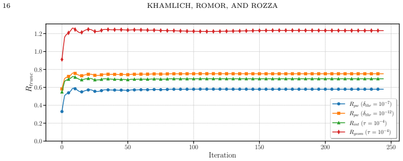
- The epsilon-scaling schedule lets a single run produce solutions across a range of regularization parameters, and the regularized potentials converge to the unregularized SOT solution as epsilon goes to zero, with relative error around 8.0e-4 at epsilon about 1e-4 in the reported test.
- Nested algorithms that require repeated RSOT solves, such as Wasserstein barycenters, Lloyd-type quantization, and shape registration, inherit the acceleration directly.
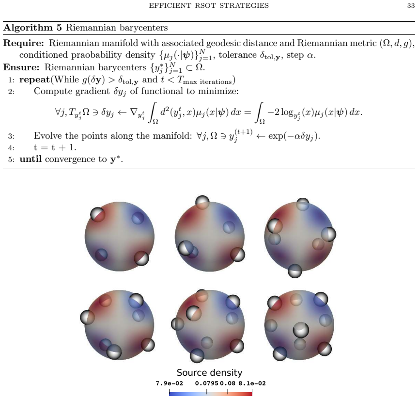
- The framework extends to non-Euclidean squared-geodesic costs, as demonstrated by blue-noise sampling on a sphere with a manifold-aware Lloyd iteration.
Reading between the lines
- The speedup claim is contingent on the softmax refinement formula being an accurate warm start; the paper neither derives it nor gives an error bound, so a reader should treat the 175x figure as heuristic rather than certified.
- A per-quadrature-point adaptive truncation radius, rather than a single global cutoff, could recover the speed of the aggressive pointwise strategy while keeping the convergence guarantee of the geometric bound.
- Because the expensive kernel evaluation is the same one that dominates fully discrete regularized OT, the truncation-plus-spatial-index acceleration is a natural candidate for GPU kernels, and the paper's preliminary GPU results suggest the CPU-only timings understate what is achievable on accelerator hardware.
- The demonstrated convergence of psi*_epsilon to the unregularized potential psi*_0 suggests the solver can serve as a robust continuation engine toward the unregularized transport plan, which matters for applications such as optical design that live in the epsilon-to-zero limit.
Editorial analysis
A structured set of objections, weighed in public.
Referee Report
Summary. The paper proposes a suite of numerical strategies for solving entropy-regularized semi-discrete optimal transport (RSOT) problems in which the continuous source measure is discretized by finite elements. The main components are: (i) adaptive truncation of the Gibbs kernel using pointwise, integral, or geometric cutoffs, accelerated by R-tree spatial queries; (ii) multilevel schemes that coarsen the source mesh, the target measure, or both, with a softmax refinement formula (Eq. (25)) for transferring potentials between target levels; and (iii) epsilon-scaling for continuation toward small regularization parameters. The authors report wall-clock speedups of up to 175x on a 116,305-point target problem, and demonstrate the framework on Wasserstein barycenters, shape registration, and blue noise sampling. An open-source C++ implementation based on deal.II and Kokkos is provided.
Significance. If the reported speedups are accompanied by verified accuracy, this would be a practically important contribution to computational optimal transport, enabling RSOT at scales relevant to PDE-constrained applications. The paper has clear strengths: the code is released, the benchmarks are extensive and use non-trivial PDE-derived densities, and the truncation bounds in Appendix B are derived from first principles rather than fitted. The convergence study in Section 6.1.3 provides a falsifiable check that the regularized solution approaches the unregularized one. However, the central claim of large-scale speedup currently lacks an accuracy validation at the scale where the speedup is reported, and the softmax refinement that drives the multilevel acceleration is asserted without a derivation or error bound. These gaps must be closed before the performance claims can be fully credited.
major comments (3)
- [Section 6.1.2, Table 3] The headline 175x speedup on the 116,305-point problem is reported as wall-clock time and fine-level iteration counts, but no accuracy metric is given for the solutions produced at this scale. The only relative error Erel (Eq. (27)) appears in Table 1 for a 14,761-point problem and compares truncation strategies against a no-truncation discretization of the same functional; it does not compare the multilevel solver against an untruncated or independently computed reference. Without such a comparison, the reported speedup cannot be separated from the possibility that the adaptive truncation and early stopping accept a less accurate solution. I recommend adding an end-to-end accuracy check at the large scale, for example by computing the untruncated dual functional value at the final multilevel potential, or by comparing against a reference solution on the fine level obtained with a more conservative tolerance.
- [Section 4.1, Eq. (23), Appendix B] The geometric truncation bound is derived for a fixed potential psi, but the implementation updates Cgeom during L-BFGS iterations using the current M, m, and J_eps(psi); Figure 3 shows the cutoff varying across iterations. Consequently, the stopping criterion ||grad J_trunc(psi)||_1 <= delta_tol certifies only the gradient of a truncated functional that changes along the optimization path. Appendix B provides no bound on ||grad J_eps - grad J_trunc|| and no bound on the distance between the minimizer of the truncated and the full functional. This is load-bearing because the multilevel speedup is measured in iterations to satisfy the truncated gradient criterion, not the gradient of the original objective. The paper should either prove a uniform-in-psi truncation error estimate or empirically demonstrate that the truncation error in the gradient remains controlled throughout the optimization.
- [Section 5.2, Eq. (25)] The softmax refinement formula is asserted without derivation. The text calls it 'analogous to one half-step of a Sinkhorn-like iteration,' but no error estimate is given relating the produced initial guess to the minimizer on the finer level. The Target-only and Combined strategies, which deliver the largest reported speedups, rely on this warm start to achieve one or two fine-level iterations. The paper should provide a derivation showing that Eq. (25) is the epsilon-smoothed c-transform of the coarse potential, and ideally an error bound, or at least report the gradient norm of the warm-started solution on the fine level to substantiate the claim that it is near-optimal.
minor comments (4)
- [Table 1, Section 6.1.1] The Integral bound with tau=1e-4 for the uniform density is marked as not converging (✗) despite an Erel of 1.7e-4, and the text states that the prescribed tau is not always a direct predictor of observed Erel because D(psi,C) is estimated from the previous iteration. This means the global relative error guarantee in Eq. (21) is not enforced in practice; this limitation should be stated explicitly in Section 4.1 where the bound is introduced, not only in the note under Table 1.
- [Section 6.1.2 and Section 6.1.3] All timings are reported as single runs without a measure of variance. Since the paper draws strong quantitative conclusions such as 175x speedup and 29.5% improvement from epsilon-scaling, at least a few repeats or a statement that timings were stable would strengthen reproducibility.
- [Appendix A, proof of Theorem 3.2] The proof contains a few minor presentation issues: in the displayed estimate the term h^{2r-k}||f||_{C^{2r-k}}||rho||_1 is missing a closing parenthesis, and the equi-continuity claim is stated briefly. These do not affect the validity of the argument but should be cleaned up.
- [Throughout] There are several typos and grammatical errors, e.g., 'probablity' (Algorithm 5), 'An analogous results holdf' (Section 6.2), 'conditioned praobability' (Algorithm 5), and 'fails' for 'falls' in some places. A careful proofreading pass is needed.
Circularity Check
No circularity found: the derivation chain is self-contained, with measured speedups against internal baselines and error bounds derived from explicit assumptions rather than fitted inputs.
full rationale
The paper's central claims are computational: truncation strategies, multilevel warm starts, and wall-clock speedups. None of the reported results reduces by construction to its inputs. The reduced dual functional J_eps(psi) in Eq. (10) is the standard RSOT dual, cited to Peyré and Cuturi, and the gradient in Eq. (11) is an exact differentiation of that functional; there is no fitted parameter renamed as a prediction. The truncation bounds in Appendix B are derived from explicit inequalities (log(1+z) <= z, uniform lower bounds on the truncated sum), giving Cint and Cgeom as sufficient conditions for a prescribed relative error tau; these are mathematical consequences, not fits. The apparent self-reference in Cgeom depending on J_eps(psi) is an implementation/correctness caveat, not a circular derivation: the bound is stated for the exact functional, and the paper explicitly says D(psi,C) is estimated from the previous iteration for Cint. The multilevel speedup (Table 3) is an empirical comparison against the paper's own single-level baseline, which is a legitimate benchmark, and the softmax refinement formula (Eq. 25) is presented as a heuristic warm-start derived from the c-transform and Sinkhorn-type updates, not as a prediction forced by a fit. The paper also validates against an external ground-truth SOT solver (Geogram power diagrams) in Section 6.1.3. Self-citations in the reference list are not load-bearing for any of the paper's theorems or numerical claims. The closest concern—that the softmax warm start lacks a rigorous error bound—is a completeness or robustness issue, not circularity. No circular steps satisfy the evidentiary standard of quoting a specific reduction of Eq. X to Eq. Y by construction.
Assumptions & free parameters
free parameters (6)
- truncation tolerance tau =
1e-4 (default); 1e-5, 1e-6 tested
- L-BFGS gradient tolerance delta_tol =
1e-3 (benchmarks), 1e-5 (barycenter inner solves)
- regularization parameter epsilon =
1e-2 (benchmarks, blue noise), 5e-6 (barycenter/registration)
- number of multilevel levels =
5 (benchmark), 4 (barycenter/registration)
- Lloyd damping theta =
0.5
- epsilon-scaling intermediate steps Ns =
1 to 3 (tested)
assumptions (5)
- standard math Strong duality and the reduction to the finite-dimensional dual J_epsilon(psi) hold for the entropy-regularized problem (Eq. 10).
- domain assumption The integrands f and g_i in Eq. (17) are sufficiently smooth, f, g_i in C^{max(k+1,2r-k)}.
- domain assumption Potentials are globally bounded, m <= psi_j <= M, and the minimum target weight nu is positive.
- standard math The source and target measures are normalized (mu(Omega)=1, sum nu_j=1).
- standard math Standard FE approximation error estimates for rho_h (Eq. 13) hold.
Cite this review
Pith. "Pith review of Efficient Numerical Strategies for Entropy-Regularized Semi-Discrete Optimal Transport." pith.science (2026). https://pith.science/paper/HJ6ADCXV
@misc{pith2026250723602,
  author       = {Pith},
  title        = {Pith review of: Efficient Numerical Strategies for Entropy-Regularized Semi-Discrete Optimal Transport},
  year         = {2026},
  howpublished = {\url{https://pith.science/paper/HJ6ADCXV}},
  note         = {Machine review of arXiv:2507.23602}
}
read the original abstract
Semi-discrete optimal transport (SOT), which maps a continuous probability measure to a discrete one, is a fundamental problem with wide-ranging applications. Entropic regularization is often employed to solve the SOT problem, leading to a regularized (RSOT) formulation that can be solved efficiently via its convex dual. However, a significant computational challenge emerges when the continuous source measure is discretized via the finite element (FE) method to handle complex geometries or densities, such as those arising from solutions to Partial Differential Equations (PDEs). The evaluation of the dual objective function requires dense interactions between the numerous source quadrature points and all target points, creating a severe bottleneck for large-scale problems. This paper presents a cohesive framework of numerical strategies to overcome this challenge. We accelerate the dual objective and gradient evaluations by combining distance-based truncation with fast spatial queries using R-trees. For overall convergence, we integrate multilevel techniques based on hierarchies of both the FE source mesh and the discrete target measure, alongside a robust scheduling strategy for the regularization parameter. When unified, these methods drastically reduce the computational cost of RSOT, enabling its practical application to complex, large-scale scenarios. We provide an open-source C++ implementation of this framework, built upon the deal.II finite element library, available at https://github.com/SemiDiscreteOT/SemiDiscreteOT.
Figures


Figures from the paper (16 more)



Reference graph
Works this paper leans on
-
[1]
Barycenters in the Wasserstein Space
Martial Agueh and Guillaume Carlier. “Barycenters in the Wasserstein Space”. In: SIAM Journal on Mathematical Analysis43.2 (Jan. 2011), pp. 904–924.doi: 10.1137/100805741
-
[2]
Luca Ambrogioni, Umut Guclu, and Marcel van Gerven. Wasserstein variational gradient descent: From semi-discrete optimal transport to ensemble variational inference. 2019. arXiv: 1811.02827 [stat.ML]
work page Pith review arXiv 2019
-
[3]
Gradient Flows in Metric Spaces and in the Space of Probability Measures
Luigi Ambrosio, Nicola Gigli, and Giuseppe Savaré. Gradient Flows in Metric Spaces and in the Space of Probability Measures. 2. ed. Lectures in Mathematics ETH Zürich. OCLC: 254181287. Birkhäuser, 2008
work page 2008
-
[4]
Automated fault detection without seismic processing
Mauricio Araya-Polo et al. “Automated fault detection without seismic processing”. In:The Leading Edge36.3 (Mar. 2017), pp. 208–214.doi: 10.1190/tle36030208.1
-
[5]
Voronoi diagrams—a survey of a fundamental geometric data struc- ture
Franz Aurenhammer. “Voronoi diagrams—a survey of a fundamental geometric data struc- ture”. In:ACM Computing Surveys23.3 (Sept. 1991), pp. 345–405.doi: 10.1145/116873. 116880
-
[6]
Minkowski-type theorems and least-squares clustering
Franz Aurenhammer, Friedrich Hoffmann, and Boris Aronov. “Minkowski-type theorems and least-squares clustering”. In:Algorithmica 20.1 (1998), pp. 61–76.doi: 10.1007/PL00009187
-
[7]
Fatima Antarou Ba and Michael Quellmalz. “Accelerating the Sinkhorn Algorithm for Sparse Multi-Marginal Optimal Transport via Fast Fourier Transforms”. In:Algorithms 15.9 (Aug. 2022), p. 311.doi: 10.3390/a15090311
-
[8]
deal.II—A general-purpose object-oriented finite element library
W. Bangerth, R. Hartmann, and G. Kanschat. “deal.II—A general-purpose object-oriented finite element library”. In:ACM Trans. Math. Softw.33.4 (Aug. 2007), 24–es.doi: 10.1145/ 1268776.1268779
arXiv 2007
Show all 76 references
-
[9]
A Newton Algorithm for Semidiscrete Optimal Transport with Storage Fees
Mohit Bansil and Jun Kitagawa. “A Newton Algorithm for Semidiscrete Optimal Transport with Storage Fees”. In:SIAM Journal on Optimization31.4 (Jan. 2021), pp. 2586–2613.doi: 10.1137/20m1357226
2021 doi
-
[10]
A hierarchical O(N log N) force-calculation algorithm
Josh Barnes and Piet Hut. “A hierarchical O(N log N) force-calculation algorithm”. In:Nature 324.6096 (Dec. 1986), pp. 446–449.doi: 10.1038/324446a0
1986 doi
-
[11]
Iterative Bregman Projections for Regularized Transportation Problems
Jean-David Benamou et al. “Iterative Bregman Projections for Regularized Transportation Problems”. In:SIAM Journal on Scientific Computing37.2 (Jan. 2015), A1111–A1138.doi: 10.1137/141000439
2015 doi
-
[12]
Auction algorithms for network flow problems: A tutorial introduc- tion
Dimitri P. Bertsekas. “Auction algorithms for network flow problems: A tutorial introduc- tion”. In:Computational Optimization and Applications1.1 (Oct. 1992), pp. 7–66.doi: 10. 1007/bf00247653
1992
-
[13]
A survey of Optimal Transport for Computer Graphics and Computer Vision
Nicolas Bonneel and Julie Digne. “A survey of Optimal Transport for Computer Graphics and Computer Vision”. In:Computer Graphics Forum42.2 (May 2023), pp. 439–460.doi: 10.1111/cgf.14778
2023 doi
-
[14]
Brenner and L
Susanne C. Brenner and L. Ridgway Scott. The Mathematical Theory of Finite Element Methods. Springer New York, 2008.doi: 10.1007/978-0-387-75934-0
2008 doi
-
[15]
Anisotropic power diagrams for polycrystal modelling: Efficient generation of curved grains via optimal transport
M. Buze et al. “Anisotropic power diagrams for polycrystal modelling: Efficient generation of curved grains via optimal transport”. In:Computational Materials Science245 (Oct. 2024), p. 113317. doi: 10.1016/j.commatsci.2024.113317
2024
-
[16]
A Fast Adaptive Multipole Algorithm for Particle Simulations
J. Carrier, L. Greengard, and V. Rokhlin. “A Fast Adaptive Multipole Algorithm for Particle Simulations”. In: SIAM Journal on Scientific and Statistical Computing 9.4 (July 1988), pp. 669–686. doi: 10.1137/0909044. REFERENCES 35
1988 doi
-
[17]
An Interpolating Distance Between Optimal Transport and Fisher–Rao Metrics
Lénaïc Chizat et al. “An Interpolating Distance Between Optimal Transport and Fisher–Rao Metrics”. In: Foundations of Computational Mathematics18.1 (Oct. 2016), pp. 1–44. doi: 10.1007/s10208-016-9331-y
2016 doi
-
[18]
Philippe G. Ciarlet. The Finite Element Method for Elliptic Problems. Society for Industrial and Applied Mathematics, 2002.doi: 10.1137/1.9780898719208. eprint: https://epubs. siam.org/doi/pdf/10.1137/1.9780898719208
2002 doi
-
[19]
Optimal Transport for Domain Adaptation
Nicolas Courty et al. “Optimal Transport for Domain Adaptation”. In:IEEE Transactions on Pattern Analysis and Machine Intelligence39.9 (Sept. 2017), pp. 1853–1865.doi: 10. 1109/tpami.2016.2615921
2017
-
[20]
Sinkhorn Distances: Lightspeed Computation of Optimal Transport
Marco Cuturi. “Sinkhorn Distances: Lightspeed Computation of Optimal Transport”. In: Advances in Neural Information Processing Systems. Ed. by C.J. Burges et al. Vol. 26. Curran Associates, Inc., 2013
2013
-
[21]
Solving semi-discrete optimal transport problems: star shapedeness and Newton’s method
Luca Dieci and Daniyar Omarov. “Solving semi-discrete optimal transport problems: star shapedeness and Newton’s method”. In:Numerical Algorithms 99.2 (Aug. 2024), pp. 949–
2024
-
[22]
Multicellular simulations with shape and volume constraints using optimal transport
Antoine Diez and Jean Feydy. Multicellular simulations with shape and volume constraints using optimal transport. 2024. arXiv:2402.17086 [q-bio.QM]
2024 arXiv
-
[23]
Centroidal Voronoi Tessellations: Appli- cations and Algorithms
Qiang Du, Vance Faber, and Max Gunzburger. “Centroidal Voronoi Tessellations: Appli- cations and Algorithms”. In:SIAM Review 41.4 (Jan. 1999), pp. 637–676.doi: 10.1137/ s0036144599352836
1999
-
[24]
Analyse de données géométriques, au delà des convolutions
Jean Feydy. “Analyse de données géométriques, au delà des convolutions”. PhD thesis. Uni- versité Paris-Saclay, 2020
2020
-
[25]
Interpolating between Optimal Transport and MMD using Sinkhorn Diver- gences
Jean Feydy et al. “Interpolating between Optimal Transport and MMD using Sinkhorn Diver- gences”. In:Proceedings of the Twenty-Second International Conference on Artificial Intelli- gence and Statistics.Ed.byKamalikaChaudhuriandMasashiSugiyama.Vol.89.Proceedings of Machine Lea...
2019
-
[26]
Sample Complexity of Sinkhorn Divergences
Aude Genevay et al. “Sample Complexity of Sinkhorn Divergences”. In:International Con- ference on Artificial Intelligence and Statistics. 2018
2018
-
[27]
Stochastic Optimization for Large-scale Optimal Transport
Aude Genevay et al. “Stochastic Optimization for Large-scale Optimal Transport”. In:Ad- vances in Neural Information Processing Systems. Ed. by D. Lee et al. Vol. 29. Curran Associates, Inc., 2016
2016
-
[28]
Wasserstein Generative Adversarial Network (WGAN)
Mehdi Ghayoumi. “Wasserstein Generative Adversarial Network (WGAN)”. In:Generative Adversarial Networks in Practice. Chapman and Hall/CRC, Nov. 2023, pp. 401–435.doi: 10.1201/9781003281344-13
2023 doi
-
[29]
Blue noise through optimal transport
Fernando de Goes et al. “Blue noise through optimal transport”. In:ACM Transactions on Graphics 31.6 (Nov. 2012), pp. 1–11.doi: 10.1145/2366145.2366190
2012
-
[30]
Power particles: an incompressible fluid solver based on power diagrams
Fernando de Goes et al. “Power particles: an incompressible fluid solver based on power diagrams”. In: ACM Transactions on Graphics34.4 (July 2015), pp. 1–11.doi: 10.1145/ 2766901
2015
-
[31]
A fast algorithm for particle simulations
L Greengard and V Rokhlin. “A fast algorithm for particle simulations”. In:Journal of Com- putational Physics 73.2 (Dec. 1987), pp. 325–348.doi: 10.1016/0021-9991(87)90140-9
1987 doi
-
[32]
Variational principles for Minkowski type problems, discrete optimal transport, and discrete Monge–Ampère equations
Xianfeng Gu et al. “Variational principles for Minkowski type problems, discrete optimal transport, and discrete Monge–Ampère equations”. In:Asian Journal of Mathematics20.2 (2016), pp. 383–398.doi: 10.4310/ajm.2016.v20.n2.a7
2016 doi
-
[33]
R-trees: a dynamic index structure for spatial searching
Antonin Guttman. “R-trees: a dynamic index structure for spatial searching”. In:ACM SIG- MOD Record14.2 (June 1984), pp. 47–57.doi: 10.1145/971697.602266
1984
-
[34]
Optimal Mass Transport for Registration and Warping
Steven Haker et al. “Optimal Mass Transport for Registration and Warping”. In: Inter- national Journal of Computer Vision 60.3 (Dec. 2004), pp. 225–240. doi: 10 . 1023 / b : visi.0000036836.66311.97
2004
-
[35]
Computer Simulation Using Particles
R.W Hockney and J.W Eastwood. Computer Simulation Using Particles. CRC Press, Mar
-
[36]
Billion-scale similarity search with GPUs
Jeff Johnson, Matthijs Douze, and Hervé Jégou. “Billion-scale similarity search with GPUs”. In: IEEE Transactions on Big Data7.3 (2019), pp. 535–547
2019
-
[37]
The Variational Formulation of the Fokker–Planck Equation
Richard Jordan, David Kinderlehrer, and Felix Otto. “The Variational Formulation of the Fokker–Planck Equation”. In: SIAM Journal on Mathematical Analysis 29.1 (Jan. 1998), pp. 1–17. doi: 10.1137/s0036141096303359
1998 doi
-
[38]
On the translocation of masses
Leonid Vitalyevich Kantorovich. “On the translocation of masses”. In: Doklady Akademii Nauk SSSR37 (1942), pp. 199–201.doi: 10.1287/mnsc.5.1.1. 36 REFERENCES
1942 doi
-
[39]
Optimal transport-based displacement interpolation with data aug- mentation for reduced order modeling of nonlinear dynamical systems
Moaad Khamlich et al. “Optimal transport-based displacement interpolation with data aug- mentation for reduced order modeling of nonlinear dynamical systems”. In:Journal of Com- putational Physics 531 (June 2025), p. 113938.doi: 10.1016/j.jcp.2025.113938
2025
-
[40]
Optimization by Simulated Annealing
S. Kirkpatrick, C. D. Gelatt, and M. P. Vecchi. “Optimization by Simulated Annealing”. In: Science 220.4598 (May 1983), pp. 671–680.doi: 10.1126/science.220.4598.671
1983 doi
-
[41]
Convergence of a Newton algorithm for semi-discrete optimal transport
Jun Kitagawa, Quentin Mérigot, and Boris Thibert. “Convergence of a Newton algorithm for semi-discrete optimal transport”. In:Journal of the European Mathematical Society21.9 (2019), pp. 2603–2651.doi: 10.4171/JEMS/889
2019 doi
-
[42]
A Comparison of Methods for Generating Poisson Disk Dis- tributions
Ares Lagae and Philip Dutré. “A Comparison of Methods for Generating Poisson Disk Dis- tributions”. In:Computer Graphics Forum27.1 (Oct. 2007), pp. 114–129.doi: 10.1111/j. 1467-8659.2007.01100.x
2007
-
[43]
A survey of the Schrödinger problem and some of its connections with optimal transport
Christian Léonard. “A survey of the Schrödinger problem and some of its connections with optimal transport”. In:Discrete & Continuous Dynamical Systems - A34.4 (2014), pp. 1533–
2014
-
[44]
A Numerical Algorithm for L2 Semi-Discrete Optimal Transport in 3D
Bruno Lévy. “A Numerical Algorithm for L2 Semi-Discrete Optimal Transport in 3D”. In: ESAIM: Mathematical Modelling and Numerical Analysis49.6 (Nov. 2015), pp. 1693–1715. doi: 10.1051/m2an/2015055
2015
-
[45]
Variational Anisotropic Surface Meshing with Voronoi Parallel Linear Enumeration
Bruno Lévy and Nicolas Bonneel. “Variational Anisotropic Surface Meshing with Voronoi Parallel Linear Enumeration”. In:Proceedings of the 21st International Meshing Roundtable. Ed. by Xiangmin Jiao and Jean-Christophe Weill. Berlin, Heidelberg: Springer Berlin Hei- delberg, 20...
2013 doi
-
[46]
Notions of optimal transport theory and how to imple- ment them on a computer
Bruno Lévy and Erica L. Schwindt. “Notions of optimal transport theory and how to imple- ment them on a computer”. In:Computers &; Graphics72 (May 2018), pp. 135–148.doi: 10.1016/j.cag.2018.01.009
2018 doi
-
[47]
Multilevel Optimal Transport: A Fast Approximation of Wasserstein-1 Distances
Jialin Liu et al. “Multilevel Optimal Transport: A Fast Approximation of Wasserstein-1 Distances”. In: SIAM Journal on Scientific Computing43.1 (Jan. 2021), A193–A220. doi: 10.1137/18m1219813
2021 doi
-
[48]
On centroidal voronoi tessellation—energy smoothness and fast computa- tion
Yang Liu et al. “On centroidal voronoi tessellation—energy smoothness and fast computa- tion”. In:ACM Trans. Graph.28.4 (Sept. 2009).doi: 10.1145/1559755.1559758
2009
-
[49]
Plugin estimation of smooth optimal transport maps
Tudor Manole et al. “Plugin estimation of smooth optimal transport maps”. In:The Annals of Statistics 52.3 (June 2024).doi: 10.1214/24-aos2379
2024 doi
-
[50]
A Convexity Principle for Interacting Gases
Robert J. McCann. “A Convexity Principle for Interacting Gases”. In:Advances in Mathe- matics 128.1 (June 1997), pp. 153–179.doi: 10.1006/aima.1997.1634
1997
-
[51]
A Multiscale Approach to Optimal Transport
Quentin Mérigot. “A Multiscale Approach to Optimal Transport”. In: Computer Graphics Forum 30.5 (Aug. 2011), pp. 1583–1592.doi: 10.1111/j.1467-8659.2011.02032.x
2011
-
[52]
Mémoiresurlathéoriedesdéblaisetdesremblais
GaspardMonge.“Mémoiresurlathéoriedesdéblaisetdesremblais”.In: Histoire de l’Académie Royale des Sciences(1781)
-
[53]
Optimal Transport with Proximal Splitting
Nicolas Papadakis, Gabriel Peyré, and Edouard Oudet. “Optimal Transport with Proximal Splitting”. In: SIAM Journal on Imaging Sciences7.1 (Jan. 2014), pp. 212–238. doi: 10. 1137/130920058
2014
-
[54]
Computational Optimal Transport: With Applications to Data Science
Gabriel Peyré and Marco Cuturi. “Computational Optimal Transport: With Applications to Data Science”. In:Foundations and Trends® in Machine Learning11.5–6 (2019), pp. 355–
2019
-
[55]
On the computation of Wasserstein barycenters
Giovanni Puccetti, Ludger Rüschendorf, and Steven Vanduffel. “On the computation of Wasserstein barycenters”. In:SSRN Electronic Journal(2018). doi: 10.2139/ssrn.3276147
2018 doi
-
[56]
Wasserstein Blue Noise Sampling
Hongxing Qin et al. “Wasserstein Blue Noise Sampling”. In:ACM Transactions on Graphics 36.5 (Oct. 2017), pp. 1–13.doi: 10.1145/3119910
2017 doi
-
[57]
Francesco Romor et al.Data assimilation performed with robust shape registration and graph neural networks: application to aortic coarctation. 2025. arXiv:2502.12097 [math.NA]
2025 arXiv
-
[58]
LearningDeepOptimalEmbeddingswithSinkhornDivergences
SoumavaKumarRoyetal.“LearningDeepOptimalEmbeddingswithSinkhornDivergences”. In: SSRN Electronic Journal(2022). doi: 10.2139/ssrn.4038042
2022 doi
-
[59]
Geometrical optics and optimal transport
Jacob Rubinstein and Gershon Wolansky. “Geometrical optics and optimal transport”. In: Journal of the Optical Society of America A34.10 (Sept. 2017), p. 1817. doi: 10 . 1364 / josaa.34.001817
2017
-
[61]
Stabilized Sparse Scaling Algorithms for Entropy Regularized Trans- port Problems
Bernhard Schmitzer. “Stabilized Sparse Scaling Algorithms for Entropy Regularized Trans- port Problems”. In:SIAM Journal on Scientific Computing41.3 (Jan. 2019), A1443–A1481. doi: 10.1137/16m1106018
2019 doi
-
[62]
TetGen, a Delaunay-Based Quality Tetrahedral Mesh Generator
Hang Si. “TetGen, a Delaunay-Based Quality Tetrahedral Mesh Generator”. In:ACM Trans- actions on Mathematical Software41.2 (Feb. 2015), pp. 1–36.doi: 10.1145/2629697
2015 doi
-
[64]
Convolutional wasserstein distances: efficient optimal transportation on geometric domains
Justin Solomon et al. “Convolutional wasserstein distances: efficient optimal transportation on geometric domains”. In:ACM Transactions on Graphics34.4 (July 2015), pp. 1–11.doi: 10.1145/2766963
2015 doi
-
[65]
Semi-discrete optimal transport: hardness, regularization and numerical solution
Bahar Taşkesen, Soroosh Shafieezadeh-Abadeh, and Daniel Kuhn. “Semi-discrete optimal transport: hardness, regularization and numerical solution”. In:Mathematical Programming 199.1–2 (July 2022), pp. 1033–1106.doi: 10.1007/s10107-022-01856-x
2022 doi
-
[66]
Overrelaxed Sinkhorn–Knopp Algorithm for Regularized Optimal Transport
Alexis Thibault et al. “Overrelaxed Sinkhorn–Knopp Algorithm for Regularized Optimal Transport”. In:Algorithms 14.5 (Apr. 2021), p. 143.doi: 10.3390/a14050143
2021 doi
-
[67]
Kokkos 3: Programming Model Extensions for the Exascale Era
Christian R. Trott et al. “Kokkos 3: Programming Model Extensions for the Exascale Era”. In: IEEE Transactions on Parallel and Distributed Systems33.4 (2022), pp. 805–817.doi: 10.1109/TPDS.2021.3097283
2022
-
[68]
Optimal Transport
Cédric Villani. Optimal Transport. Springer Berlin Heidelberg, 2009.doi: 10.1007/978-3- 540-71050-9
2009 doi
-
[69]
Topics in Optimal Transportation
Cédric Villani. Topics in Optimal Transportation. American Mathematical Society, Mar
-
[70]
Self-supervised non-rigid structure from motion with improved training of Wasserstein GANs
Yaming Wang et al. “Self-supervised non-rigid structure from motion with improved training of Wasserstein GANs”. In:IET Computer Vision 17.4 (Feb. 2023), pp. 404–414.doi: 10. 1049/cvi2.12175
2023
-
[71]
Di Wu, Ling Liang, and Haizhao Yang.PINS: Proximal Iterations with Sparse Newton and Sinkhorn for Optimal Transport. 2025. arXiv:2502.03749 [cs.LG]
2025 arXiv
-
[72]
Examination of Document Clustering Based on Independent Topic Analysis and Word Embeddings
Riku Yasutomi, Seiji Yamada, and Takashi Onoda. “Examination of Document Clustering Based on Independent Topic Analysis and Word Embeddings”. In:Proceedings of the 17th International Conference on Agents and Artificial Intelligence. SCITEPRESS - Science and Technology Publicat...
2025 doi
-
[73]
Sample Elimination for Generating Poisson Disk Sample Sets
Cem Yuksel. “Sample Elimination for Generating Poisson Disk Sample Sets”. In:Computer Graphics Forum34.2 (May 2015), pp. 25–32.doi: 10.1111/cgf.12538. 38 REFERENCES Appendix A. Proof of convergence of minimizers of regularized SOT discrete functional Proof. Standard error anal...
2015 doi
-
[607]
doi: 10.1561/2200000073
-
[1004]
doi: 10.1007/s11075-024-01903-y
-
[1574]
doi: 10.3934/dcds.2014.34.1533
2014 doi
-
[2003]
doi: 10.1090/gsm/058
-
[2021]
doi: 10.1201/9780367806934
Reviewed August 6, 2026 · model on record in the stance chip above.
Discussion (0). Continue with ORCID to comment.