REVIEW 3 major objections 5 minor 43 references
A charge model as an effective model of one-dimensional Hubbard and extended Hubbard systems: its application to linear optical spectrum calculations in large systems based upon many-body Wannier functions
T0 review · 3 major / 5 minor · reviewed 2026-08-14 · deepseek-v4-flash
Pith's one-line read An effective model that separates spin from charge reproduces the optical spectra of one-dimensional Mott insulators at realistic interaction strengths.
desk verdict A genuinely new effective model with a solid small-cluster validation; the MBWF extrapolation to large systems is heuristic and the abstract overstates the agreement, but the paper deserves refereeing. read the letter →
The pith
A machine-rendered reading of the paper's core claim, the machinery that carries it, and where it could break.
The reading
What carries the argument
The load-bearing object is the projected charge model $H^{(C)}(t)=P H(t) P$, defined on basis states in which the positions of $M$ doublons and $M$ holons are recorded while all spins are described by a single factorized wave function $f^{(M)}$, taken to be the ground state of the Heisenberg Hamiltonian with $N-2M$ sites. The key numerical input is the overlap $c_S(M)=0.82$, the thermodynamic-limit overlap between that Heisenberg ground state and the state formed by inserting a nearest-neighbor spin singlet; it renormalizes every matrix element that creates or annihilates a holon–doublon pair. The boundary twist $\theta_M=(\pi/2)\,\mathrm{mod}(N-2M,4)$ fixes the phase accumulated when a charge crosses the periodic boundary. The second mechanism is the many-body Wannier construction: the seven dominant optically active eigenstates of a 16-site cluster are unitarily rotated into spatially localized many-body states, and the resulting Hamiltonian and current matrix elements, which decay within the cluster, are extrapolated to about 200 sites.
What would settle it
Compute the charge-model optical spectrum at $U/T=3$ and compare it with dynamical DMRG: the paper already notes that the high-energy tail is underestimated and that the one-pair nature of the Wannier states degrades as $U$ decreases, so a clearly visible mismatch there would set the model's lower boundary below $U/T=5$. Alternatively, compute the exact ground-state overlap $c_S$ in the original Hubbard model at intermediate $U$; a value that departs from $0.82$ as the singlet insertion point moves would falsify the single-parameter renormalization.
Extended reading notes
Core claim
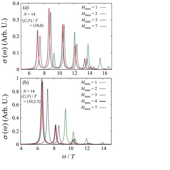
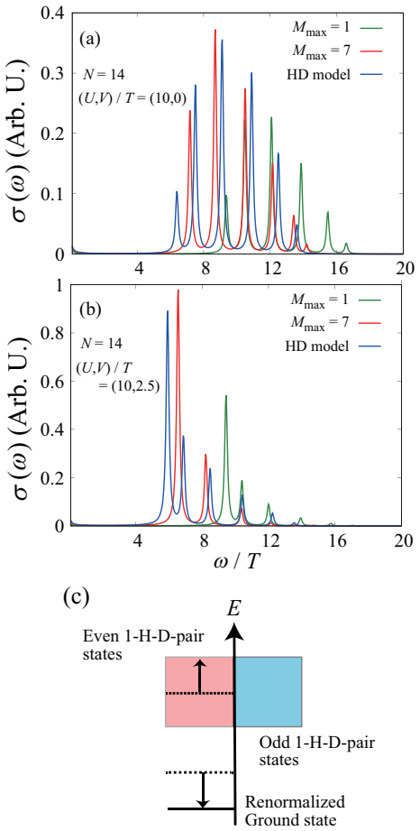
The central claim is that the effective Hamiltonian $H^{(C)}(t)=P H(t) P$, obtained by projecting the Hubbard or extended Hubbard Hamiltonian onto a subspace in which every basis state with $M$ holon–doublon pairs carries one and the same spin wave function—the ground state of the Heisenberg chain on the $N-2M$ singly occupied sites—is quantitatively faithful for linear optical response. The paper shows that all spin physics entering the projection is carried by a phase $\theta_M=(\pi/2)\,\mathrm{mod}(N-2M,4)$ and by the overlap $c_S(M)=0.82$ between a Heisenberg ground state and the state obtained by inserting a nearest-neighbor spin singlet. Within this subspace, charge fluctuations are treated exactly, and they are essential: truncating to a single H-D pair shifts the spectrum by about $0.5T$ and fails for $U/T=5$, while the full charge model matches the original models at $N=14$ and matches dynamical DMRG benchmarks for systems of about 200 sites at $U/T=10$, $6$, and $5$. The paper also claims that the many-body Wannier construction, which localizes the leading optically active eigenstates and extrapolates their Hamiltonian and current matrix elements, converges by $N\approx200$.
Load-bearing premise
The construction assumes that one and the same spin wave function, the Heisenberg ground state, is correct for every placement of holons and doublons; if the spin background rearranges around charge carriers at intermediate $U$, the projection drops the physics that controls the optical response.
Editorial extensions
If this is right
- For $U/T$ between 5 and 10 and $V/T$ up to 2.5, the charge model's Hilbert space is about 20 times smaller than the original model's, so large-system optical spectra can be computed exactly in the charge sector without repeated basis transformations.
- The holon–doublon two-particle model, which omits pair creation and annihilation, is not reliable in this regime: it misses the optical gap by about $T$ at $U/T=10$ and fails at smaller $U$.
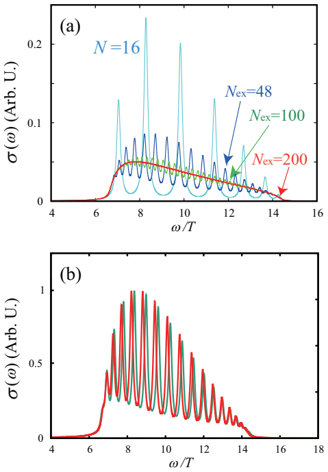
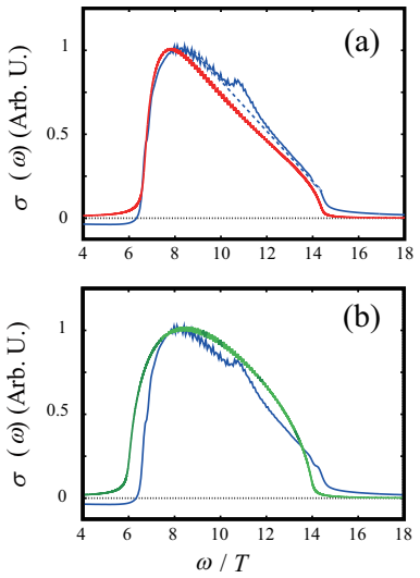
- The many-body Wannier extrapolation from a 16-site cluster yields spectra for about 200 sites whose low- and high-energy edges, peak positions, and asymmetry agree with t-DMRG and DDMRG benchmarks, meaning finite-size effects can be removed while keeping explicit excited-state wave functions.
- Because the charge model retains wave functions, spectral features can be interpreted in terms of renormalized holon–doublon distances, a type of diagnosis that is harder with repeated-basis-transformation methods.
Reading between the lines
- One extension the paper leaves implicit is to use the same projection for pump–probe response: comparing transient spectra of the charge model with those of the full Hubbard model would isolate spin-charge coupling as the driver of the photoinduced Mott-gap collapse, a comparison the authors flag as future work.
- The many-body Wannier procedure is in principle transferable to the original Hubbard and extended Hubbard models and to strongly excited states, but there the Wannier states would need to carry spin structure and the number of relevant eigenstates grows with spin-charge coupling, so the construction is not straightforward.
- A testable refinement would be to let $c_S$ depend on holon–doublon distance or on the local spin environment; the paper's observation that the shortest-distance diagonal matrix element is boundary-sensitive suggests such dependence may matter just above $V/T=2.5$.
Signed reviews
Editorial analysis
A structured set of objections, weighed in public.
Referee Report
Summary. The paper introduces a 'charge model' for the half-filled one-dimensional Hubbard and extended Hubbard models. The model is defined by projecting the full Hamiltonian onto a subspace in which spin and charge degrees of freedom are factorized: every basis state with M holon-doublon pairs carries the same spin wave function, taken to be the ground state of a Heisenberg chain with N-2M sites. Hopping matrix elements that change the number of holon-doublon pairs are renormalized by a factor cS(M)=0.82, obtained from an independent spin-chain overlap calculation. The authors validate the charge model against exact diagonalization for N=14 at U/T=10, then introduce many-body Wannier functions (MBWFs) built from the seven principal optically active eigenstates of a 16-site cluster. Matrix elements are extrapolated to larger systems, yielding optical conductivity spectra for effective sizes up to Nex=200, which are compared with t-DMRG and DDMRG results for U/T=5, 6, and 10 and for (U,V)/T=(10,2.5). The central claim is that spin-charge separation works well in the intermediate-coupling regime U=5-10T and that the MBWF extrapolation reproduces the optical spectra of the original models in large systems.
Significance. If the central claim is correct, the paper offers a practical route to optical spectra of strongly correlated 1D systems at sizes approaching the thermodynamic limit while retaining explicit wave-function information, which DMRG-based methods do not provide. The N=14 exact comparison is a genuine and useful benchmark, and the renormalization factor cS(M)=0.82 is not fitted to the optical spectra, which strengthens the model validation. The comparisons against t-DMRG and DDMRG are appropriate external checks. However, the extrapolation from a 16-site cluster to Nex=200 rests on several ad hoc truncation and averaging steps without a controlled error estimate, so the large-system part of the claim is not yet established at the level claimed in the abstract.
major comments (3)
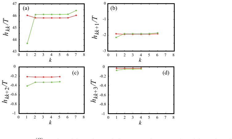
- [III B, Eqs. (19)-(21) and Appendix C] The MBWF extrapolation is the load-bearing step for the headline claim of spectra at N≈200, but it lacks any controlled convergence check. Starting from a 16-site cluster, the construction (i) retains only seven 'principal peaks' as a complete orthonormal set, (ii) sets h_{k,k+i}=0 for i≥4, (iii) replaces h_{k,k+i} for k beyond the 16-site range by constants m0-m3 averaged over k=2..6, and (iv) zero-pads the current matrix elements and rescales them by sqrt(Nex/N). None of these steps is derived from the microscopic model, and the paper does not test stability under changes in the starting cluster size (e.g., N=12 or 20) or in the number of retained peaks (e.g., 9 or 11). Without such checks, the observed agreement with DMRG at Nex=200 could reflect the flexibility of the extrapolation protocol rather than the validity of the charge model or the MBWF construction.
- [III A and Fig. 9] The abstract claims validity in the intermediate regime U=5-10T, but the direct validation of the charge model against exact diagonalization is shown only for U/T=10 and N=14 (Fig. 2). The U/T=5 and 6 comparisons in Fig. 9 are obtained by first applying the MBWF extrapolation to the charge model and then comparing with DMRG. This conflates the validity of the charge model with the validity of the extrapolation, which is precisely the uncontrolled step identified above. The text itself states that 'checks are required of the results down to U/T=5,' but no direct charge-model-versus-Hubbard exact comparison at U/T=5 or 6 is presented. A direct N=14 comparison at these values is needed before the U=5-10T claim can be supported.
- [Figs. 8-10 and Eq. (18)] All comparisons between the extrapolated charge-model spectra and the DMRG benchmarks are normalized to unit maximum, so absolute spectral weights (and hence the f-sum or total optical weight) are never compared. In addition, the t-DMRG spectrum in Fig. 10(c) is computed with an adjusted broadening γ=0.14T chosen to match the MBWF peak width, and in Fig. 8(a) the spin-derived hump around ω/T=11 is explicitly excluded from the comparison. These choices reduce the stringency of the claimed quantitative agreement. The paper should either compare absolute conductivities or clearly state that the claim concerns spectral shape only.
minor comments (5)
- [Throughout] The phrase 'zero center-of-gravity momentum' should be 'zero total momentum' or 'zero center-of-mass momentum'.
- [Fig. 2 caption] The caption states that spectra are normalized so that <g|J^† J|g>=1, whereas later figures are normalized to unit maximum; the normalization convention should be stated consistently for every figure.
- [Sec. II around Eq. (14)] The notation cS(M) is used both for the overlap in Eq. (14) and, in the following sentence, for the weight cS^2(M); please distinguish these quantities explicitly.
- [Sec. II, Eq. (2)] For M=N/2 the spin wave function f(M) is defined on zero singly occupied sites, which is a limiting case; please specify the convention used for the Heisenberg ground state when N-2M=0.
- [Appendix C, Eqs. (C1)-(C5)] The averaging ranges differ among m0, m1, m2, and m3 (e.g., m3 averages only k=2..4); a sentence explaining why these ranges are chosen would help the reader assess the extrapolation.
Circularity Check
No significant circularity: the charge model is benchmarked against exact diagonalization and DMRG, and the cS(M)=0.82 parameter comes from an independent spin-chain overlap calculation, not from fitting the optical spectra.
full rationale
The central derivation is not circular. The charge model is defined by the projected Hamiltonian H(C)=PH(t)P in a spin-charge factorized subspace (Eq. 6), and its validity is tested against quantities computed independently: exact diagonalization of the original Hubbard and extended Hubbard models at N=14 (Fig. 2) and t-DMRG/DDMRG calculations at N=80 and N=100 (Figs. 8-10). The only renormalization parameter, cS(M)=0.82, is not fitted to the optical spectra; it is taken from the thermodynamic-limit value of the overlap cS(M)=0.820+0.740(N-2M)^-2 computed for the Heisenberg chain, with the paper explicitly saying 'we adopt the value in the thermodynamic limit (cS(M)=0.82)'. The MBWF construction derives its matrix elements from a 16-site charge-model calculation and extrapolates them by the constants in Eqs. (C1)-(C5) and by truncation/rescaling of the current matrix elements; none of these constants is adjusted to match the DMRG benchmarks, so the large-system spectra are genuine predictions against external references. Adjusting the DMRG broadening in Fig. 10(c) ('we have adjusted gamma of t-DMRG by fitting') changes only the comparison width and does not feed back into the charge-model matrix elements. The paper's own caveats that 'checks are required of the results down to U/T=5' and that the method 'underestimates the tail structure on the high-energy side' are honest limitations about accuracy, not reductions of the output to the input. No load-bearing self-citation, imported uniqueness theorem, or fitted-input-called-prediction step was found.
Assumptions & free parameters
free parameters (2)
- cS(M), spin-pair overlap reduction factor =
0.82 (thermodynamic limit; size dependence fitted to 0.820 + 0.740 (N-2M)^-2)
- Number of principal peaks retained in MBWF construction =
7
assumptions (5)
- domain assumption The relevant low-energy subspace S consists of states where spin and charge degrees of freedom are exactly factorized for each number M of holon-doublon pairs.
- domain assumption For each M, the spin wave function f(M) is the ground state of the 1D Heisenberg Hamiltonian with N-2M sites, with cyclic phase exp(-i theta_M).
- domain assumption Spin-charge coupling beyond the subspace is small: (1-P)H(t)P is first order in (T/(U-V)) sqrt(1-cS^2) and at most 0.11 for the parameters used.
- ad hoc to paper The unitary matrix V^(tr)_kk' = (2/sqrt(N)) sin(2 pi k k'/N) used to construct MBWFs remains valid for interacting eigenstates with Mmax=8.
- ad hoc to paper Long-range matrix elements of the effective Hamiltonian and current operator can be extrapolated by averaging and zero-padding, with the current operator scaled by sqrt(Nex/N).
Cite this review
Pith. "Pith review of A charge model as an effective model of one-dimensional Hubbard and extended Hubbard systems: its application to linear optical spectrum calculations in large systems based upon many-body Wannier functions." pith.science (2026). https://pith.science/paper/HW7LRFGM
@misc{pith2026190809335,
  author       = {Pith},
  title        = {Pith review of: A charge model as an effective model of one-dimensional Hubbard and extended Hubbard systems: its application to linear optical spectrum calculations in large systems based upon many-body Wannier functions},
  year         = {2026},
  howpublished = {\url{https://pith.science/paper/HW7LRFGM}},
  note         = {Machine review of arXiv:1908.09335}
}
abstract
We propose an effective model called the "charge model", for the half-filled one-dimensional Hubbard and extended Hubbard models. In this model, spin-charge separation, which has been justified from an infinite on-site repulsion ($U$) in the strict sense, is compatible with charge fluctuations. Our analyses based on the many-body Wannier functions succeeded in determining the optical conductivity spectra in large systems. The obtained spectra reproduce the spectra for the original models well even in the intermediate $U$ region of $U=5-10T$, with $T$ being the nearest-neighbor electron hopping energy. These results indicate that the spin-charge separation works fairly well in this intermediate $U$ region against the usual expectation and that the charge model is an effective model that applies to actual quasi-one-dimensional materials classified as strongly correlated electron systems.
Figures


Figures from the paper (8 more)




Reference graph
Works this paper leans on
- [1]
-
[2]
J. M. Luttinger, J. Math. Phys. 4 , 1154 (1963)
work page 1963
-
[3]
D. C. Mattis and E. H. Lieb, J. Math. Phys. 6 , 304 (1965)
work page 1965
- [4]
-
[5]
F. D. M. Haldane, J. Phys. C: Solid State Phys. 14 , 2585 (1981)
work page 1981
-
[6]
H. J. Schulz, Int. J. Mod. Phys. B 5 , 57 (1991)
work page 1991
- [7]
- [8]
Show all 43 references
-
[9]
Parola and S
A. Parola and S. Sorella, Phys. Rev. Lett. 64 , 1831 (1990)
1990
-
[10]
Ogata, T
M. Ogata, T. Sugiyama, and H. Shiba, Phys. Rev. B 43 , 8401 (1991)
1991
-
[11]
B. J. Kim, H. Koh, E. Rotenberg, S.-J. Oh, H. Eisaki, N. Motoyama, S. Uchida, T, Tohyama, S. Maekawa, Z.-X. Shen, and C. Kim, Nature Physics 2 , 397 (2006)
2006
-
[12]
Kishida, H
H. Kishida, H. Matsuzaki, H. Okamoto, T. Manabe, M. Yamashita, Y. Taguchi, and Y. Tokura, Nature (London) 405 , 929 (2000)
2000
-
[13]
Mizuno, K
Y. Mizuno, K. Tsutsui, T. Tohyama, and S. Maekawa, Phys. Rev. B 62 , R4769 (2000)
2000
-
[14]
Kishida, M
H. Kishida, M. Ono, K. Miura, H. Okamoto, M. Izumi, T. Manako, M. Kawasaki, Y. Taguchi, Y. Tokura, T. Tohyama, K. Tsutsui, and S. Maekawa, Phys. Rev. Lett. 87 , 177401 (2001)
2001
-
[15]
M. Ono, K. Miura, A. Maeda, H. Matsuzaki, H. Kishida, Y. Taguchi, Y. Tokura, M. Yamashita, and H. Okamoto, Phys. Rev. B 70 , 085101 (2004)
2004
-
[16]
S. Iwai, M. Ono, A. Maeda, H. Matsuzaki, H. Kishida, H. Okamoto, and Y. Tokura, Phys. Rev. Lett. 91 , 057401 (2003)
2003
-
[17]
Okamoto, H
H. Okamoto, H. Matsuzaki, T. Wakabayashi, Y. Takahashi, and T. Hasegawa, Phys. Rev. Lett. 98 , 037401 (2007)
2007
-
[18]
Woynarovich, J
F. Woynarovich, J. Phys. C: Solid State Phys. 15 , 85 (1982)
1982
-
[19]
Parola and S
A. Parola and S. Sorella, Phys. Rev. B 45 , 13156 (1992)
1992
-
[20]
Eskes, A
H. Eskes, A. M. Ole\' s , M. B. J. Meinders, and W. Stephan, Phys. Rev. B 50 , 17980 (1994)
1994
-
[21]
K. Penc, K. Hallberg, F. Mila, and H. Shiba, Phys. Rev. B 55 , 15475 (1997)
1997
-
[22]
Stephan and K
W. Stephan and K. Penc, Phys. Rev. B 54 , R17269 (1996)
1996
-
[23]
Sorella and A
S. Sorella and A. Parola, Phys. Rev. Lett. 76 , 4604 (1996)
1996
-
[24]
Sorella and A
S. Sorella and A. Parola, Phys. Rev. B 57 , 6444 (1998)
1998
-
[25]
Lante and A
V. Lante and A. Parola, Phys. Rev. B 80 , 195113 (2009)
2009
-
[26]
Dagotto, Rev
E. Dagotto, Rev. Mod. Phys. 66 , 763 (1994)
1994
-
[27]
S. R. White, Phys. Rev. Lett. 69 , 2863 (1992)
1992
-
[28]
Jeckelmann, F
E. Jeckelmann, F. Gebhard, F. H. L. Essler, Phys, Rev. Lett. 85 , 3910 (2000)
2000
-
[29]
F. H. L. Essler, F. Gebhard, and E. Jeckelmann, Phys. Rev. B 64 , 125119 (2001)
2001
-
[30]
Jeckelmann, Phys
E. Jeckelmann, Phys. Rev. B 66 , 045114 (2002)
2002
-
[31]
Jeckelmann, Phys
E. Jeckelmann, Phys. Rev. B 67 , 075106 (2003)
2003
-
[32]
Benthien, F
H. Benthien, F. Gebhard, and E. Jeckelmann, Phys. Rev. Lett. 92 , 256401 (2004)
2004
-
[33]
Benthien, and E
H. Benthien, and E. Jeckelmann, Phys. Rev. B 75 , 205128 (2007)
2007
-
[34]
S. S. Kancharla and C. J. Bolech, Phys. Rev. B 64 , 085119 (2001)
2001
-
[35]
A. C. Tiegel, T. Veness, P. E. Dargel, A. Honecker, T. Pruschke, I. P. McCulloch, and F. H. L. Essler, Phys. Rev. B 93 , 125108 (2016)
2016
-
[36]
J. C. Talstra, S. P. Strong, and P. W. Anderson, Phys. Rev. Lett. 74 , 5256 (1995)
1995
-
[37]
Matsueda, N
H. Matsueda, N. Bulut, T. Tohyama,and S. Maekawa, Phys. Rev B 72 , 075136 (2005)
2005
-
[38]
A. S. Mishchenko and N. Nagaosa, Phys. Rev. Lett. 93 , 036402 (2004)
2004
-
[39]
Takahashi, H
A. Takahashi, H. Itoh, and M. Aihara, Phys. Rev. B 77 , 205105 (2008)
2008
-
[40]
S. R. White, and A. E. Feiguin, Phys. Rev. Lett. 93 , 076401 (2004)
2004
-
[41]
Sota, and M
S. Sota, and M. Itoh, J. Phys. Soc. Jpn. 76 , 054004 (2007)
2007
-
[42]
H. Lu, C. Shao, J. Bon c a, D. Manske, and T. Tohyama, Phys. Rev. B 91 , 245117 (2015)
2015
-
[43]
C. Shao, T. Tohyama, H.-G. Luo, and H. Lu, Phys. Rev. B 93 , 195144 (2016)
2016
Reviewed August 14, 2026 · model on record in the stance chip above.
Discussion (0). Continue with ORCID to comment.