REVIEW 2 major objections 5 minor 84 references
Efficient Sampling Allocation Strategies for General Graph-Filter-Based Signal Recovery
T0 review · 2 major / 5 minor · reviewed 2026-08-08 · deepseek-v4-flash
Pith's one-line read Choosing sensors by recovery-error cost functions rather than bandlimitedness or smoothness assumptions cuts graph-signal recovery MSE by up to 50% in underdetermined systems.
desk verdict A generally solid extension of optimal-design sampling to graph-filtered models, with a real scoping flaw in the correlated-noise claims and a convexity guarantee that does not match the implemented algorithm. read the letter →
The pith
A machine-rendered reading of the paper's core claim, the machinery that carries it, and where it could break.
The reading
What carries the argument
The object doing the work is the regularized sampled-information matrix $K(d)=\mathbf{h}_M(L)DR^{-1}D\mathbf{h}_M(L)+\mu\mathbf{h}_R^+(L)$, where $\mathbf{h}_M(L)$ is the measurement graph filter and $\mathbf{h}_R^+(L)$ is a positive-semidefinite graph filter encoding prior knowledge. The GFR-ML estimator inverts this matrix, and each proposed cost function is a tractable function of it: $\mathrm{bCRB}=\mathrm{tr}(K^{-1}\mathbf{h}_M(L)DR^{-1}D\mathbf{h}_M(L)K^{-1})$, $\mathrm{BMSE}=\mathrm{tr}(K^{-1})$, WC-MSE adds $\mu^2$ times the squared largest singular value of $K^{-1}\mathbf{h}_R^+(L)$, and WC-BMSE is $\lambda_{\min}^{-1}(K)$. The shared gradient formula $\nabla C(d)=-2\mathrm{diag}(R^{-1}D\mathbf{h}_M(L)K^{-1}QK^{-1}\mathbf{h}_M(L))$, with a different matrix $Q$ for each criterion, is what allows the alternating projected-gradient algorithm to optimize all four cost functions with the same code path, and the rank-one structure of adding one sensor is what makes the greedy updates fast.
What would settle it
Run the paper's synthetic-data Monte Carlo comparison with a correlated noise covariance such as $R_{ij}=0.5^{|i-j|}$ at $q/N=70\%$; if sensors chosen by the bCRB or BMSE criteria no longer achieve lower empirical MSE than A- and E-design, the misspecified Fisher-information model is what carries the reported gain.
Extended reading notes
Core claim
The paper's central claim is that for the underdetermined measurement model $y=\mathbf{h}_M(L)x+e$, the right sensor set is the one that minimizes the recovery error of the graph-filtered regularized maximum likelihood (GFR-ML) estimator, not a proxy tied to bandlimitedness or smoothness. Concretely, with $D=\mathrm{diag}(d)$ marking the sampled nodes, the estimator is $\hat{x}=K^{-1}(d)(\mathbf{h}_M(L)DR^{-1}Dy+\mu\mathbf{h}_R^+(L)x_0)$ with $K(d)=\mathbf{h}_M(L)DR^{-1}D\mathbf{h}_M(L)+\mu\mathbf{h}_R^+(L)$, and its MSE decomposes into a noise term plus a bias term that depends on the unknown signal $x$. Since direct MSE minimization is therefore impossible, the paper proposes four signal-independent cost functions — bCRB (a lower bound on the MSE of estimators with a prescribed bias), worst-case MSE, Bayesian MSE, and worst-case Bayesian MSE — and shows in Monte Carlo experiments that optimizing them reduces recovery MSE by up to 50% relative to A-design, E-design, and LR-design sampling.
Load-bearing premise
The load-bearing premise is that sampling a set of nodes only reweights noise through a diagonal mask, which is exact only when the noise at different nodes is uncorrelated or correlated only within known groups; with general correlated noise, the bCRB and the four cost functions built on it are misspecified.
Editorial extensions
If this is right
- A fixed sensor budget buys lower recovery error: in the tested scenarios the proposed designs match or beat A-, E-, and LR-design, so the same accuracy can be obtained with fewer measurements.
- Bandlimited and smooth signal models become special cases: under strict bandlimitedness with $\mu\to\infty$, the bCRB and BMSE reduce to A-design and the WC-BMSE reduces to E-design.
- For diagonal noise, adding a sensor is a rank-one update of $K(d)$, reducing the greedy algorithm's total cost to $O(qN^3)$ or $O(qN^2)$ instead of $O(qN^4)$.
- The alternating projected-gradient solver scales the criteria to large graphs, demonstrated on a 2,642-node road network.
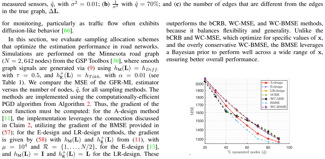
- In the power-system experiments, bCRB-based sampling is the most robust to noise and topology mismatch, while BMSE and WC-BMSE give the best average performance in Bayesian settings.
Reading between the lines
- Because the proposed costs collapse to A- and E-design in the exact-bandlimited limit, the relative advantage should be largest under model mismatch; a direct test is whether the gap shrinks as signals approach perfect bandlimitedness.
- The bCRB and the derived costs treat the Fisher information as $\mathbf{h}_M(L)DR^{-1}D\mathbf{h}_M(L)$, which is exact for diagonal or block-diagonal noise; re-deriving them with the exact observed covariance would extend the same machinery to correlated noise, a regime the reported experiments (all with $R=\sigma^2 I$) do not test.
- With polynomial or Chebyshev-approximated graph filters, the matrix-vector products in $K(d)$ are local, so the same sampling criteria could plausibly run in a distributed way on much larger networks.
Editorial analysis
A structured set of objections, weighed in public.
Referee Report
Summary. This paper considers the recovery of graph signals from partial noisy observations under a linear graph-filter measurement model y = hM(L)x + e, with a regularization term ||x - x0||^2_{h_R^+(L)}. It introduces the GFR-ML estimator in Eqs. (14)-(15) and proposes four sampling-allocation cost functions: the biased Cramér-Rao bound (bCRB), the worst-case MSE (WC-MSE), the Bayesian MSE (BMSE), and the worst-case Bayesian MSE (WC-BMSE). Two solvers are presented: a greedy algorithm with efficient rank-one updates, and an alternating projected gradient descent (PGD) algorithm based on a convex relaxation. The paper reports Monte Carlo simulations on synthetic graphs, the IEEE 118-bus power system, and the Minnesota road network, showing up to 50% MSE reduction relative to A-design, E-design, and LR-design sampling.
Significance. The paper offers a potentially unifying task-based framework for sampling in graph-signal recovery, with bandlimited and smoothness-based designs arising as special cases. The authors supply explicit gradient expressions and complexity analyses for both solvers, and the empirical evaluation spans synthetic data and two realistic network datasets. If the theoretical claims are restricted to diagonal/white noise (as used in all experiments) or corrected for general R, the framework is a useful contribution. The rank-one update formulas in Eqs. (41)-(44) and the gradient expressions in Claim 3 are practical assets.
major comments (2)
- [Section IV-A, Eqs. (20)-(25)] The paper states in Eq. (21) that Dy ~ N(DhM(L)x, R) for the partial-observation model in Eq. (9). This is incorrect for a general noise covariance R: the noise term De has covariance D R D, so the correct distribution is Dy ~ N(DhM(L)x, D R D). Consequently, the FIM in Eq. (22), the bCRB in Eq. (25), and the MSE expression in Eq. (20) are valid only when D and R commute (in particular, for diagonal R), because the simplification D R^{-1} D R D R^{-1} D = D R^{-1} D is used implicitly. All experiments in Section VI use R = sigma^2 I or R = 0.01I, so the numerical MSE comparisons are not invalidated; however, the general claims about arbitrary noise covariance in the abstract and in Sections III and IV need to be corrected or explicitly restricted to diagonal or block-diagonal R.
- [Section V-B2 and Appendix H] The convexity proof in Appendix H establishes convexity of tr(K_affine(w)^{-1}) and lambda_max(K_affine(w)^{-1}) in the reparameterized variables w_i = d_i^2, with K_affine(w) defined in Eq. (124). However, Algorithm 2 performs projected gradient descent directly on d, using the gradient with respect to d from Claim 3 and the projections in Eqs. (52)-(53) on d. Convexity in w does not imply convexity in d, so the stated global-convergence guarantee does not apply to the implemented algorithm. The sentence in Section V-B2 that PGD 'is expected to converge to the global optimum' should either be softened or the algorithm should be reparameterized and implemented in the w-variables.
minor comments (5)
- [Eq. (20)] The derivation of Eq. (20) mentions that the covariance of De is D R D, but the displayed trace term contains D R^{-1} D; please add the intermediate expression D R^{-1} D R D R^{-1} D and state explicitly where diagonal R is assumed.
- [Supplement, Appendix B] The supplement refers to 'Theorem 1 in [67]', where [67] is the arXiv version of this same paper; this should be replaced by an internal cross-reference to the paper's own Theorem 1.
- [Algorithm 1] The input list says 'number of nodes, q', but q denotes the number of selected sensors; please correct the label.
- [Fig. 1 caption] The caption item '(3) hM(L) = hDiff' should read '(c) hM(L) = hDiff' to match the panels.
- [Section V-B, Eqs. (48)-(53)] The backtracking line search in Eq. (48) uses the projection P defined in Eq. (49), which is a projection onto the non-convex binary set, but the actual update in Eq. (50) and the projection steps in Eqs. (52)-(53) use the relaxed convex set. This inconsistency should be fixed so that the line search condition matches the projection actually applied in the update.
Circularity Check
No circularity found: the GFR-ML estimator and the four sampling cost functions are derived algebraically from the stated model, and the simulated MSE reductions are evaluated by Monte Carlo rather than by fitting.
full rationale
The paper's derivation chain is self-contained. The GFR-ML estimator in Eqs. (14)-(15) follows by differentiating the convex objective in Eq. (13); the error expression in Eq. (19) and the MSE in Eq. (20) are algebraic consequences of the model and estimator. The bCRB in Eq. (25), the WC-MSE in Eq. (26), the BMSE in Eq. (29), and the WC-BMSE in Eq. (30) are each derived from Eq. (20) or from the stated Gaussian model, with no parameter fitted to the quantities later reported as improvements. The A-design/E-design/LR-design comparisons in Section VI are Monte Carlo evaluations, not predictions manufactured from the proposed cost functions. The self-citations to the authors' prior work ([2], [6], [7], [67]) identify special cases and extended context but do not supply the central claim; no load-bearing result rests on an unverified self-citation. A separate correctness concern, not a circularity, is that Eq. (21) states Dy ~ N(Dh_M(L)x, R) whereas Eqs. (9) and the MSE derivation in Eq. (20) imply that the covariance of De is D R D; for non-diagonal R the printed FIM and cost functions do not match the actual partial-observation model. All simulations use diagonal R (sigma^2 I or 0.01I), so the reported empirical reductions are not forced by construction. Accordingly, no circular step is present.
Assumptions & free parameters
free parameters (4)
- regularization parameter mu =
0.1 in simulations
- reference signal x0 =
not estimated; implicitly zero in most experiments
- worst-case ball radius in WC-MSE =
1
- assumed bandlimited frequency set R for A/E baselines =
{1,...,N/2} in most simulations
assumptions (6)
- standard math The graph Laplacian is diagonalizable as L = V diag(lambda) V^{-1} with V^T = V^{-1} for an undirected graph.
- domain assumption The measurement filter hM(L) and regularizer hR(L) are known graph filters, and hR(L) is positive semidefinite.
- domain assumption The noise is zero-mean Gaussian with known covariance R.
- domain assumption The Bayesian prior is x ~ N(x0, (1/mu) hR(L)^dag), with the pseudo-inverse as the covariance.
- domain assumption For Theorem 1, the blocks U_R^T K_M U_R and U_{V\R}^T hR U_{V\R} are invertible.
- domain assumption R is diagonal for the submodularity and convexity results.
Cite this review
Pith. "Pith review of Efficient Sampling Allocation Strategies for General Graph-Filter-Based Signal Recovery." pith.science (2026). https://pith.science/paper/I65ZYE4B
@misc{pith2026250205583,
  author       = {Pith},
  title        = {Pith review of: Efficient Sampling Allocation Strategies for General Graph-Filter-Based Signal Recovery},
  year         = {2026},
  howpublished = {\url{https://pith.science/paper/I65ZYE4B}},
  note         = {Machine review of arXiv:2502.05583}
}
abstract
Sensor placement plays a crucial role in graph signal recovery in underdetermined systems. In this paper, we present the graph-filtered regularized maximum likelihood (GFR-ML) estimator of graph signals, which integrates general graph filtering with regularization to enhance signal recovery performance under a limited number of sensors. Then, we investigate task-based sampling allocation aimed at minimizing the mean squared error (MSE) of the GFR-ML estimator by wisely choosing sensor placement. Since this MSE depends on the unknown graph signals to be estimated, we propose four cost functions for the optimization of the sampling allocation: the biased Cram$\acute{\text{e}}$r-Rao bound (bCRB), the worst-case MSE (WC-MSE), the Bayesian MSE (BMSE), and the worst-case BMSE (WC-BMSE), where the last two assume a Gaussian prior. We investigate the properties of these cost functions and develop two algorithms for their practical implementation: 1) the straightforward greedy algorithm; and 2) the alternating projection gradient descent (PGD) algorithm that reduces the computational complexity. Simulation results on synthetic and real-world datasets of the IEEE 118-bus power system and the Minnesota road network demonstrate that, in the tested scenarios, the proposed sampling allocation methods reduce the MSE by up to $50\%$ compared to the common sampling methods A-design, E-design, and LR-design. Thus, the proposed methods improve the estimation performance and reduce the required number of measurements in graph signal processing (GSP)-based signal recovery in the case of underdetermined systems.
Figures


Reference graph
Works this paper leans on
-
[1]
Newman, Networks: An Introduction
M. Newman, Networks: An Introduction . New Y ork, NY , USA: Oxford University Press, Inc., 2010
2010
-
[2]
State estima tion in partially observable power systems via graph signal proces sing tools,
L. Dabush, A. Kroizer, and T. Routtenberg, “State estima tion in partially observable power systems via graph signal proces sing tools,” Sensors, vol. 23, no. 3, p. 1387, 2023
2023
-
[3]
Stankovi´ c, D
L. Stankovi´ c, D. P . Mandic, M. Dakovi´ c, M. Brajovi´ c, B. Scalzo, S. Li, and A. G. Constantinides, Data Analytics on Graphs Part II: Signals on Graphs . now, 2020
2020
-
[4]
Three-dimensional struct ure determination from common lines in cryo-EM by eigenvectors and semidefinit e programming,
A. Singer and Y . Shkolnisky, “Three-dimensional struct ure determination from common lines in cryo-EM by eigenvectors and semidefinit e programming,” SIAM journal on imaging sciences , vol. 4, no. 2, pp. 543–572, 2011
2011
-
[5]
Distributed clock synchron ization over wireless networks: Algorithms and analysis,
A. Giridhar and P . R. Kumar, “Distributed clock synchron ization over wireless networks: Algorithms and analysis,” in IEEE CDC , Dec. 2006, pp. 4915–4920
work page 2006
-
[6]
Detection of false data in jection attacks in smart grids based on graph signal processing,
E. Drayer and T. Routtenberg, “Detection of false data in jection attacks in smart grids based on graph signal processing,” IEEE Syst. J. , vol. 14, no. 2, pp. 1886–1896, 2020
work page 2020
-
[7]
V erifying the smoothness of graph signals: A graph signal processing approach,
L. Dabush and T. Routtenberg, “V erifying the smoothness of graph signals: A graph signal processing approach,” IEEE Trans. Signal Process., vol. 72, pp. 4349–4365, 2024
work page 2024
-
[8]
Identifica tion of outages in power systems with uncertain states and optimal s ensor locations,
Y . Zhao, J. Chen, A. Goldsmith, and H. V . Poor, “Identifica tion of outages in power systems with uncertain states and optimal s ensor locations,” IEEE J. Sel. Topics Signal Process. , vol. 8, no. 6, pp. 1140–1153, 2014
work page 2014
Show all 84 references
-
[9]
The emerging field of signal processing on grap hs: Extend- ing high-dimensional data analysis to networks and other ir regular do- mains,
D. I. Shuman, S. K. Narang, P . Frossard, A. Ortega, and P . V an- dergheynst, “The emerging field of signal processing on grap hs: Extend- ing high-dimensional data analysis to networks and other ir regular do- mains,” IEEE Signal Process. Mag., vol. 30, no. 3, pp. 83–98, May 2013
2013
-
[10]
Discrete signal proc essing on graphs: Frequency analysis,
A. Sandryhaila and J. M. F. Moura, “Discrete signal proc essing on graphs: Frequency analysis,” IEEE Trans. Signal Process. , vol. 62, no. 12, pp. 3042–3054, June 2014
2014
-
[11]
Efficient sampling set selection for bandlimited graph signals using graph spectral proxies,
A. Anis, A. Gadde, and A. Ortega, “Efficient sampling set selection for bandlimited graph signals using graph spectral proxies,” IEEE Trans. Signal Process. , vol. 64, no. 14, pp. 3775–3789, 2016
2016
-
[12]
A distributed tracking algo rithm for reconstruction of graph signals,
X. Wang, M. Wang, and Y . Gu, “A distributed tracking algo rithm for reconstruction of graph signals,” IEEE J. Sel. Topics Signal Process. , vol. 9, no. 4, pp. 728–740, June 2015
2015
-
[13]
Discrete signal processing on graphs: Sampling theory,
S. Chen, R. V arma, A. Sandryhaila, and J. Kovaˇ cevi´ c, “ Discrete signal processing on graphs: Sampling theory,” IEEE Trans. Signal Process. , vol. 63, no. 24, pp. 6510–6523, Dec. 2015
2015
-
[14]
Local measurement and recon struction for noisy bandlimited graph signals,
X. Wang, J. Chen, and Y . Gu, “Local measurement and recon struction for noisy bandlimited graph signals,” Signal Process. , pp. 119–129, Dec. 2016
2016
-
[15]
Samp ling of graph signals with successive local aggregations,
A. G. Marques, S. Segarra, G. Leus, and A. Ribeiro, “Samp ling of graph signals with successive local aggregations,” IEEE Trans. Signal Process., vol. 64, no. 7, pp. 1832–1843, Apr. 2016
2016
-
[16]
Sampli ng signals on graphs: From theory to applications,
Y . Tanaka, Y . C. Eldar, A. Ortega, and G. Cheung, “Sampli ng signals on graphs: From theory to applications,” IEEE Signal Process. Mag. , vol. 37, no. 6, pp. 14–30, 2020
2020
-
[17]
Line ar-time sampling on signed graphs via Gershgorin disc perfect align ment,
C. Dinesh, S. Bagheri, G. Cheung, and I. V . Baji´ c, “Line ar-time sampling on signed graphs via Gershgorin disc perfect align ment,” in Proc. of ICASSP , 2022, pp. 5942–5946
2022
-
[18]
Global and local uncertainty principles for signals on graphs,
N. Perraudin, B. Ricaud, D. I. Shuman, and P . V anderghey nst, “Global and local uncertainty principles for signals on graphs,” APSIPA Transactions on Signal and Information Processing , vol. 7, p. e3, 2018
2018
-
[19]
Fast resampling of three-dimensional point clouds via graphs,
S. Chen, D. Tian, C. Feng, A. V etro, and J. Kovaˇ cevi´ c, “ Fast resampling of three-dimensional point clouds via graphs,” IEEE Trans. Signal Process., vol. 66, no. 3, pp. 666–681, 2018
2018
-
[20]
Random sampling of bandlimited signals on graphs,
G. Puy, N. Tremblay, R. Gribonval, and P . V andergheynst , “Random sampling of bandlimited signals on graphs,” Applied and Computational Harmonic Analysis , vol. 44, no. 2, pp. 446–475, 2018
2018
-
[21]
Cheby shev polynomial approximation for distributed signal processi ng,
D. I. Shuman, P . V andergheynst, and P . Frossard, “Cheby shev polynomial approximation for distributed signal processi ng,” in Proc. of DCOSS , 2011, pp. 1–8
2011
-
[22]
Introduction to graph signal processing
A. Ortega, “Introduction to graph signal processing.” Cambridge University Press, 2022
2022
-
[23]
Distribute d algorithm for graph signal inpainting,
S. Chen, A. Sandryhaila, and J. Kovacevic, “Distribute d algorithm for graph signal inpainting,” in Proc. of ICASSP, April 2015, pp. 3731–3735
2015
-
[24]
Reco nstruction of graph signals through percolation from seeding nodes,
S. Segarra, A. G. Marques, G. Leus, and A. Ribeiro, “Reco nstruction of graph signals through percolation from seeding nodes,” IEEE Trans. Signal Process. , vol. 64, no. 16, pp. 4845–4860, August 2016
2016
-
[25]
F ast graph sampling set selection using gershgorin disc alignment,
Y . Bai, F. Wang, G. Cheung, Y . Nakatsukasa, and W. Gao, “F ast graph sampling set selection using gershgorin disc alignment,” IEEE Trans. Signal Process. , vol. 68, pp. 2419–2434, 2020
2020
-
[26]
Sampling graph signa ls with sparse dictionary representation,
K. Zhang, M. Coutino, and E. Isufi, “Sampling graph signa ls with sparse dictionary representation,” in Proc. of EUSIPCO , 2021, pp. 1815–1819
2021
-
[27]
Sampling of g raph signals via randomized local aggregations,
D. V alsesia, G. Fracastoro, and E. Magli, “Sampling of g raph signals via randomized local aggregations,” IEEE Trans. Signal Inf. Process. Netw., vol. 5, no. 2, pp. 348–359, 2019
2019
-
[28]
Sampling of graph signals with succes sive aggregations based on graph fractional fourier transform,
D. Wei and Z. Y an, “Sampling of graph signals with succes sive aggregations based on graph fractional fourier transform, ” Digital Signal Processing, vol. 136, p. 103970, 2023
2023
-
[29]
Generalized sampling of multi-dimensional graph signals based on prior information,
——, “Generalized sampling of multi-dimensional graph signals based on prior information,” Signal Processing, vol. 224, p. 109601, 2024
2024
-
[30]
Compressed sampling in s hift-invariant spaces associated with frft,
H. Zhao, L. Zhang, and L. Qiao, “Compressed sampling in s hift-invariant spaces associated with frft,” IEEE Access , pp. 166 081–166 094, 2021
2021
-
[31]
Generalized Sampling on Grap hs With Subspace and Smoothness Priors,
Y . Tanaka and Y . C. Eldar, “Generalized Sampling on Grap hs With Subspace and Smoothness Priors,” IEEE Trans. Signal Process. , vol. 68, pp. 2272–2286, 2020
2020
-
[32]
Sensor selection via convex optim ization,
S. Joshi and S. Boyd, “Sensor selection via convex optim ization,” IEEE Trans. Signal Process. , vol. 57, no. 2, pp. 451–462, 2009
2009
-
[33]
Sparsity-promoting sensor s election for non-linear measurement models,
S. P . Chepuri and G. Leus, “Sparsity-promoting sensor s election for non-linear measurement models,” IEEE Trans. Signal Process. , vol. 63, no. 3, pp. 684–698, 2015
2015
-
[34]
Sensor management b ased on convex optimization via pcrlb and joint interception pro bability,
Y . Liu, L. Zhou, Q. Wei, and B. Zhao, “Sensor management b ased on convex optimization via pcrlb and joint interception pro bability,” in 2022 IEEE Sensors , 2022, pp. 1–4. 14
2022
-
[35]
Power systems test case archive
“Power systems test case archive.” [Online]. Availabl e: http://www.ee.washington.edu/research/pstca/
-
[36]
GSPBOX: A toolbox for signal processing on graphs,
N. Perraudin, J. Paratte, D. Shuman, L. Martin, V . Kalof olias, P . V andergheynst, and D. K. Hammond, “GSPBOX: A toolbox for signal processing on graphs,” ArXiv e-prints , Aug. 2014
2014
-
[37]
Signal recovery on graphs: V ariation minimization,
S. Chen, A. Sandryhaila, J. M. F. Moura, and J. Kovaˇ cevi ´ c, “Signal recovery on graphs: V ariation minimization,” IEEE Trans. Signal Process., vol. 63, no. 17, pp. 4609–4624, Sept. 2015
2015
-
[38]
Graph signal processing: Overview, cha llenges, and applications,
A. Ortega, P . Frossard, J. Kovaˇ cevi´ c, J. M. F. Moura, a nd P . V andergheynst, “Graph signal processing: Overview, cha llenges, and applications,” Proc. IEEE , vol. 106, no. 5, pp. 808–828, May 2018
2018
-
[39]
Bridgin g hydraulics and graph signal processing: A new perspective t o estimate water distribution network pressures,
X. Zhou, S. Liu, W. Xu, K. Xin, Y . Wu, and F. Meng, “Bridgin g hydraulics and graph signal processing: A new perspective t o estimate water distribution network pressures,” W ater Research, vol. 217, p. 118416, 2022
2022
-
[40]
Consensus filters for sensor networks and distributed sensor fusion,
R. Olfati-Saber and J. S. Shamma, “Consensus filters for sensor networks and distributed sensor fusion,” in Proceedings of the 44th IEEE Conference on Decision and Control , Dec. 2005, pp. 6698–6703
2005
-
[41]
Graph signal processing for machine learning: A review and new per spectives,
X. Dong, D. Thanou, L. Toni, M. Bronstein, and P . Frossar d, “Graph signal processing for machine learning: A review and new per spectives,” IEEE Signal Process. Mag. , vol. 37, no. 6, pp. 117–127, 2020
2020
-
[42]
How to learn a graph from smooth signals ,
V . Kalofolias, “How to learn a graph from smooth signals ,” in Journal of Machine Learning Research (JMLR) , 2016, pp. 920–929
2016
-
[43]
Signal recovery on graphs: Fundamental limits of sampling strategies,
S. Chen, R. V arma, A. Singh, and J. Kovaˇ cevi´ c, “Signal recovery on graphs: Fundamental limits of sampling strategies,” IEEE Trans. Signal Inf. Process. Netw. , vol. 2, no. 4, pp. 539–554, 2016
2016
-
[44]
Learnin g Laplacian matrix from bandlimited graph signals,
L. O. B. Le Bars, P . Humbert and A. Kalogeratos, “Learnin g Laplacian matrix from bandlimited graph signals,” In Proc. of ICASSP , pp. 2937–2941, 2019
2019
-
[45]
Learning Laplacian matrix in smooth graph signal representations,
X. Dong, D. Thanou, P . Frossard, and P . V andergheynst, “ Learning Laplacian matrix in smooth graph signal representations,” IEEE Trans. Signal Process. , vol. 64, no. 23, pp. 6160–6173, Dec. 2016
2016
-
[46]
Graph topology learning and signal recovery via Bayesian inference
M. Ramezani-Mayiami, M. Hajimirsadeghi, K. Skretting , R. S. Blum, and H. V . Poor, “Graph topology learning and signal recovery via Bayesian inference.” in DSW, 2019, pp. 52–56
2019
-
[47]
Lecture notes on ridge regression ,
W. N. van Wieringen, “Lecture notes on ridge regression ,” 2015. [Online]. Available: https://arxiv.org/abs/1509.09169
2015 arXiv
-
[48]
Energy ef ficient WSN: a cross-layer graph signal processing solution to info rmation redundancy,
A. Chiumento, N. Marchetti, and I. Macaluso, “Energy ef ficient WSN: a cross-layer graph signal processing solution to info rmation redundancy,” in In Proc. of ISWCS , 2019, pp. 645–650
2019
-
[49]
S. M. Kay, Fundamentals of statistical signal processing: Estimatio n Theory. Englewood Cliffs (N.J.): Prentice Hall PTR, 1993, vol. 1
1993
-
[50]
Exploring estim ator bias-variance tradeoffs using the uniform cr bound,
A. O. Hero, J. A. Fessler, and M. Usman, “Exploring estim ator bias-variance tradeoffs using the uniform cr bound,” IEEE Trans. Signal Process., vol. 44, no. 8, pp. 2026–2041, 1996
2026
-
[51]
Minimum variance in biased estimation: Bo unds and asymptotically optimal estimators,
Y . C. Eldar, “Minimum variance in biased estimation: Bo unds and asymptotically optimal estimators,” IEEE Trans. Signal Process. , vol. 52, no. 7, pp. 1915–1930, 2004
1915
-
[52]
R. A. Horn and C. R. Johnson, Matrix Analysis , 2nd ed. New Y ork, NY , USA: Cambridge University Press, 2012
2012
-
[53]
Big data analytic s using graph signal processing,
F. Amin, O. M. Barukab, and G. S. Choi, “Big data analytic s using graph signal processing,” Computers, Materials and Continua , vol. 74, no. 1, pp. 489–502, 2022
2022
-
[54]
The matrix cookbook,
K. B. Petersen and M. S. Pedersen, “The matrix cookbook, ” Techn. Univ. Denmark, vol. 7, no. 15, p. 510, 2012
2012
-
[55]
D. P . Bertsekas, Nonlinear Programming , 2nd ed. Athena Scientific, 1999
1999
-
[56]
Boyd and L
S. Boyd and L. V andenberghe, Convex Optimization. New Y ork, NY , USA: Cambridge University Press, 2004
2004
-
[57]
Alternating projections,
S. Boyd and J. Dattorro, “Alternating projections,” EE392o, Stanford University, 2003
2003
-
[58]
Graph filt ers for signal processing and machine learning on graphs,
E. Isufi, F. Gama, D. I. Shuman, and S. Segarra, “Graph filt ers for signal processing and machine learning on graphs,” IEEE Trans. Signal Process., pp. 1–32, 2024
2024
-
[59]
N. L. R. Y . Bengio, O. Delalleau, Semi-Supervised Learning . United States of America: Massachusetts Institute of Technology, 2006
2006
-
[60]
Learn ing heat diffusion graphs,
D. Thanou, X. Dong, D. Kressner, and P . Frossard, “Learn ing heat diffusion graphs,” IEEE Trans. Signal Inf. Process. Netw. , vol. 3, no. 3, pp. 484–499, 2017
2017
-
[61]
Source loca lization on graphs via l1 recovery and spectral graph theory,
R. Pena, X. Bresson, and P . V andergheynst, “Source loca lization on graphs via l1 recovery and spectral graph theory,” in 2016 IEEE 12th Image, Video, and Multidimensional Signal Processing W orkshop (IVMSP), 2016, pp. 1–5
2016
-
[62]
Learning to identify sources of net work diffusion,
C. Y e and G. Mateos, “Learning to identify sources of net work diffusion,” in Proc. of EUSIPCO , 2022, pp. 727–731
2022
-
[63]
Grid-graph signal pr ocessing (grid-GSP): A graph signal processing framework for the pow er grid,
R. Ramakrishna and A. Scaglione, “Grid-graph signal pr ocessing (grid-GSP): A graph signal processing framework for the pow er grid,” IEEE Trans. Signal Process. , vol. 69, pp. 2725–2739, 2021
2021
-
[64]
Monitoring and optimization for power grids: A signal processing perspective,
G. B. Giannakis, V . Kekatos, N. Gatsis, S. J. Kim, H. Zhu, and B. F. Wollenberg, “Monitoring and optimization for power grids: A signal processing perspective,” IEEE Signal Process. Mag. , vol. 30, no. 5, pp. 107–128, Sept. 2013
2013
-
[65]
Towards modeling the traffic data on road networks,
U. Demiryurek, B. Pan, F. Banaei-Kashani, and C. Shahab i, “Towards modeling the traffic data on road networks,” in Proc. of IWCTS . New Y ork, NY , USA: Association for Computing Machinery, 2009, p. 13–18
2009
-
[66]
Characterizing diffusion processes in city traffic,
P . Medina, S. C. Carrasco, M. S. Jofr´ e, J. Rogan, and J. A . V aldivia, “Characterizing diffusion processes in city traffic,” Chaos, Solitons & Fractals, vol. 165, p. 112846, 2022
2022
-
[67]
Efficient sampling alloc ation strategies for general graph-filter-based signal recovery ,
L. Dabush and T. Routtenberg, “Efficient sampling alloc ation strategies for general graph-filter-based signal recovery ,” arXiv preprint arXiv:2502.05583, 2025
2025 arXiv
-
[68]
On submodu larity and controllability in complex dynamical networks,
T. H. Summers, F. L. Cortesi, and J. Lygeros, “On submodu larity and controllability in complex dynamical networks,” IEEE Transactions on Control of Network Systems , vol. 3, no. 1, pp. 91–101, 2016. Supplemental Material for the Paper: Efficient Sampling Allocation Strategies ...
2016
-
[69]
15 regularizer from ( 78), it is required that ε = 0, corresponding to the limit µ → ∞
with the prior x0 and the 1In fact, the derivation and the results in this section are th e same for any filter that satisfy h+ R (λ i) = 0 , ∀i ∈ R . 15 regularizer from ( 78), it is required that ε = 0, corresponding to the limit µ → ∞. Thus, under these assumptions, our gene...
-
[71]
To proceed, we multiply both sides of (
for µ→∞ becomes (see Theorem 1 in [ 67]) V−1K†(d)V = [ (UT RKMUR)−1 0 0 0 ] , (82) where KM △ = hM(L)DR−1DhM(L), (83) and UT RKMUR is a non-singular matrix. To proceed, we multiply both sides of (
-
[77]
into ( 30) gives BMSEW C(d) = λmax ( (UT RKMUR)−1 ) . (99) Notably, when h+ R (L) is full column rank, which corre- sponds mathematically toV\R =V in ( 94), ( 94) yields a de- generate case in which the estimator relies solely on the pri or and becomes independent of the obser...
-
[79]
(111) Since both A and E defined in (
and the property that h+ R (L)UR = 0, one can verify that V−1K(d)V is a block matrix of the form given in ( 100), where A = UT RKMUR, B = U−1 R KMUV\R , D = UT V\R KMUV\R , E = UT V\R h+ R (L)UV\R . (111) Since both A and E defined in (
-
[80]
Moreover, in the strictly bandlimited case, the signal lies in the subspace spanned by UR, and thus the effect of the regularization term in K†(d) vanishes
can be written as ˆ ˜xR = PRV−1K−1(d) hT M(L)DR−1Dy = UT RK−1(d) hT M(L)DR−1Dy, (81) where we use the fact that UR = VPT R, and PRV−1 = UT R. Moreover, in the strictly bandlimited case, the signal lies in the subspace spanned by UR, and thus the effect of the regularization te...
-
[82]
Substituting (
by PR from the left and by V−1 from the right to obtain UT RK†(d) = ( UT RKMUR)−1UT R, (84) where we used the property that the columns of V−1K†(d)V correspond to the complement of the bandlimited subspace are zero. Substituting (
-
[83]
(115) Proof: For anyS⊆V and diagonal R, it follows that hM(L)DR−1DhM(L) = ∑ i∈S 1 Ri,i [hM(L)]V,i [hM(L)]T V,i
can be written as K(1S∪{a}) = K(1S) + KM(1{a}), (114) where all the contribution of the nodes in {a} is captured by KM(1{a}) = ∑ i∈{a} R−1 i,i [hM(L)]V,i [hM(L)]T V,i . (115) Proof: For anyS⊆V and diagonal R, it follows that hM(L)DR−1DhM(L) = ∑ i∈S 1 Ri,i [hM(L)]V,i [hM(L)]T V...
-
[84]
(85) Now, we define the effective measurement matrix as HR ≜ hM(L)UR∈ RN ×|R|
into the estimator ( 81) results in ˆ ˜xR = ( UT RKMUR ) −1 UT RhT M(L)DR−1Dy. (85) Now, we define the effective measurement matrix as HR ≜ hM(L)UR∈ RN ×|R|. (86) Using this definition and ( 82), we obtain UT RKMUR = HT RDR−1DHR, UT RhT M(L) = HT R, which implies that (
-
[85]
can be rewritten as ˆ ˜xR = ( HT RDR−1DHR ) −1 HT RDR−1y. (87) The corresponding vertex-domain estimator ˆx ∈ RN is obtained by projecting the estimated GFT coefficients in ( 87) back to the vertex domain using the bandlimited eigenbasis UR. Thus, we have ˆx = UR ˆ ˜xR = UR ( H...
-
[86]
as an equivalent maximization by negating the objective S∗ = arg max S⊆V , |S|=q −BMSE(1S), (118) and prove these properties for the resulting negative objec tive. We begin with defining the derived set function fa : 2 V\{a}→ R for the negative BMSE ∀{a}∈V as fa(S) =− tr ( K−1(...
-
[102]
along with the definitions in ( 111), we obtain the result in ( 109). Finally, since the limit in ( 109) exists and is finite, the limit of the matrix product limµ →∞ V−1µ2h+ R (L)K†(d)K†(d)h+ R (L)V can be evaluated by multiplying the limit matrices obtained in ( 109). This yie...
-
[103]
Moreover, using matrix multiplication rules, we have M−1(µ) [ 0 0 0 µE ] = [ 0 −µA−1B S−1(µ)E 0 µS−1(µ)E ]
and using ( 106), each term involving S−1(µ) vanishes, yielding the result in (101). Moreover, using matrix multiplication rules, we have M−1(µ) [ 0 0 0 µE ] = [ 0 −µA−1B S−1(µ)E 0 µS−1(µ)E ] . (107) Taking the limit µ→∞ and applying ( 106), we obtain the result in ( 102). Now...
-
[108]
(98) Similarly, substituting (
into ( 29), we obtain BMSE(d) = tr((UT RKMUR)−1). (98) Similarly, substituting (
-
[110]
(97) By substituting (
into ( 26) without constant terms yields MSEW C(d) = bCRB(d) +λmax ( UT V\R KMUR ( UT RKMUR ) −2 UT RKMUV\R ) . (97) By substituting (
-
[111]
Consider the expression V−1µK†(d)h+ R (L)V = V−1µK†(d)VV−1h+ R (L)V
are invertible, ( 101) from Theorem 1 directly implies the result in ( 108). Consider the expression V−1µK†(d)h+ R (L)V = V−1µK†(d)VV−1h+ R (L)V. (112) Note that by using the assumption that h+ R (L)UR = 0 and substituting the notations in ( 111), we have V−1h+ R (L)V = [ 0 0 ...
-
[116]
for the set S∪{ a}, with {a} /∈S , into (15), we obtain K(1S∪{a}) = ∑ i∈S∪{a} 1 Ri,i [hM(L)]V,i [hM(L)]T V,i + µh+ R (L) = K(1S) + ∑ i∈{a} R−1 i,i [hM(L)]V,i [hM(L)]T V,i . APPENDIX G: P ROVE OF SUBMODULARITY OF THE BMSE In this section, we show that the negative BMSE cost fun...
Reviewed August 8, 2026 · model on record in the stance chip above.
Discussion (0). Continue with ORCID to comment.