REVIEW 3 major objections 5 minor 21 references
Analytical solutions for the Extracellular-Membrane-Intracellular model
T0 review · 3 major / 5 minor · reviewed 2026-08-16 · deepseek-v4-flash
Pith's one-line read This paper derives exact reference solutions for the Extracellular-Membrane-Intracellular cardiac model and verifies that a mortar finite-element solver reproduces them under refinement.
desk verdict The single-cell and N-cell manufactured benchmarks are usable, but the two-cell exact solution as printed does not satisfy the EMI equations, so the paper's strongest new claim needs correction. read the letter →
The pith
A machine-rendered reading of the paper's core claim, the machinery that carries it, and where it could break.
The reading
What carries the argument
The machinery is separation of variables under radial symmetry, plus the method of manufactured solutions for the Cartesian case. In the radial problems, assuming the potentials depend only on the radius reduces the Laplace equations to one-dimensional integrals, and the equal-conductivity assumption makes the interface flux condition reduce to equality of the leading integration constants; the remaining constants are fixed by the ordinary differential equations for the passive membrane and gap-junction potentials. In the manufactured solution, the spatial factor $X = \cos(2\pi x/\alpha_g)\cos(2\pi y/\beta_g)\cos(2\pi z/\gamma_g)$ is chosen so that $\nabla X \cdot \hat{n} = 0$ on all interior interfaces, which trivializes the normal-flux coupling, while the time factors are exponentials and forcing terms are added to make the potentials satisfy Poisson equations and the passive cell models.
What would settle it
Substitute equations (11), (13), and (14) into the original interface conditions (4b) and (4d): in every case the normal-flux term vanishes because $\nabla X \cdot \hat{n} = 0$, so the solutions are exact for zero-flux data. To test whether they serve as a general benchmark, construct an EMI problem with a nonzero constant normal flux on a membrane and check whether any member of these families can satisfy it; the continuity condition shows no member can, so the family's validity is restricted to the zero-flux case.
Extended reading notes
Core claim
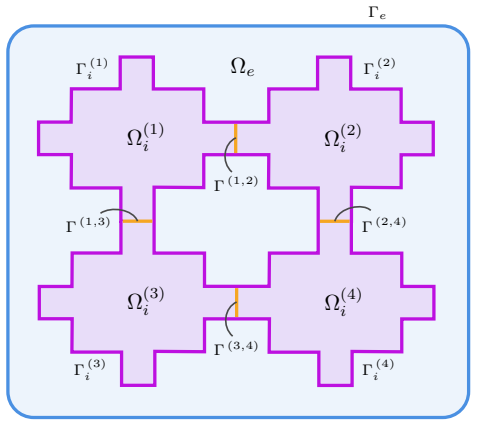
The central claim is that equations (11), (13), and (14) are valid analytical and manufactured solutions of the EMI model with passive cell models, and that they are usable as benchmark references. The first family solves a single radially symmetric cell in polar coordinates; the second solves two coupled radially symmetric semi-spherical cells in spherical coordinates; both require equal intracellular and extracellular conductivities. The third is a true manufactured solution for N identical cuboidal cells in Cartesian coordinates, built by separation of variables with a cosine profile whose normal derivative vanishes on every membrane and gap junction, together with explicit forcing terms. Numerical experiments with the mortar finite element method and operator splitting reproduce all three sets of solutions, with L2 errors that decrease under mesh and time-step refinement.
Load-bearing premise
The load-bearing premise is that a solution with zero normal flux across all membranes and gap junctions is enough to verify an EMI solver, because the proposed benchmarks never exercise the coupling currents that distinguish the EMI model from a set of decoupled diffusion problems.
Editorial extensions
If this is right
- EMI solver developers can use these solutions as convergence benchmarks for spatial and temporal discretization in both two and three dimensions.
- The single-cell and two-cell families provide time-dependent reference data, so they test time integrators and operator-splitting error in addition to spatial accuracy.
- The manufactured solution works for any number N of cells in a sheet, allowing scaling tests and parallel implementations to be checked against a known answer.
- Because the benchmark family covers coupled cells and gap junctions, it goes beyond the previous single-cell manufactured solutions used in the EMI literature.
Reading between the lines
- Because every constructed solution has zero normal flux across membranes and gap junctions, a solver that mishandles the flux-coupling interface conditions could still pass all three benchmarks; a test that enforces a nonzero transmembrane current is still needed.
- Extending the derivation to unequal intracellular and extracellular conductivities, or to anisotropic conductivities, would produce benchmarks that actually exercise the transmembrane current, which none of the current solutions do.
- One could adapt the manufactured-solution construction to a spatial factor with nonzero normal derivative and solve the resulting consistency condition on the time factors; the paper's zero-flux choice is sufficient for verification but not necessary.
Signed reviews
Editorial analysis
A structured set of objections, weighed in public.
Referee Report
Summary. The paper presents three families of reference solutions for the EMI model of cardiac electrophysiology: a single two-dimensional cell solution in polar coordinates, a two-cell solution in spherical coordinates, and an N-cell manufactured solution in Cartesian coordinates. For each it gives a derivation, parameter restrictions, and a numerical experiment using a mortar finite-element/operator-splitting implementation. The stated goal is to provide exact benchmarks that EMI solver codes should reproduce.
Significance. The single-cell family is clean and self-consistent: with the stated parameter choices, Eq. (11) satisfies the Laplace equations, the membrane relation v = u_i - u_e, and the initial condition, and it exercises a nonzero membrane current. The manufactured solution is a standard MMS construction with explicit forcing, and the accompanying code and data are publicly available. However, the two-cell family in Eq. (13) is not correct as printed, the Experiment 2 formulas do not satisfy the EMI interface conditions, and none of the benchmarks exercises the gap-junction current coupling. The paper therefore has a useful core but cannot currently be used as a reliable reference for EMI verification.
major comments (3)
- [Section 3.2, after Eq. (13l)] The statement that w=(v0^(1)-v0^(2))e^{-t/(C_m R_m)} satisfies the gap-junction IVP (12j)-(12k) in the case v0^(1)≠v0^(2), w0=0 is inconsistent: at t=0 the expression equals v0^(1)-v0^(2)≠0, not w0=0. The correct compatibility condition is w0=v0^(1)-v0^(2), w_rest=0, and C_m^(1,2)R_m^(1,2)=C_mR_m. As printed, the derivation of Eq. (13) does not establish a valid family for unequal initial transmembrane potentials.
- [Section 5.2.2, Eqs. (12d), (12e), (12g)] The printed Experiment 2 formulas do not solve the EMI model. At ρ=5 and t=0, u_i^(2)-u_e = 2, whereas the printed v^(2) equals 1954/181≈10.8, and the stated initial value v0^(2)=30 is not reproduced. The normal derivatives also fail (12d): ∂ρ u_e = -2e^{-t/10}cos(t) while ∂ρ u_i^(2) = -0.4e^{-t/10}cos(t), so the membrane flux balance is violated by a factor of 5. Consequently, Eq. (13) is not verified by Experiment 2, and the error norms in Table 2 are not errors against a solution of the stated problem.
- [Section 3.3, after Eq. (14e)] The manufactured solution is constructed with ∇X·n=0 on all membranes and gap junctions, so I_m^(k)=I_m^(k,ℓ)=0 on every interface. This means Experiment 3 verifies only the volume equations and the membrane/gap-junction ODEs with zero normal-flux coupling; it does not exercise the transmission conditions (4b) and (4d) that distinguish the EMI model from decoupled Poisson problems. The abstract's claim that the solutions verify 'the accuracy of numerical simulations of the EMI model' should be tempered to state this scope limitation explicitly.
minor comments (5)
- [Section 3.2, Eq. (13l)] The superscript w^(2,1) is used here while the system is written for w^(1,2); standardize the notation.
- [Figure 6 caption] The caption repeats u_i^(2) twice; it should refer to u_i^(1) and u_i^(2).
- [Table 1] The table contains spacing artifacts such as '5 .929' and '2 .736'; please reformat the error entries.
- [Section 5.2.3] The gap-junction resistance R_m^(k,l) is not specified, although the choice g^(k,l)=0 with w=(k-l)e^{-t}X implicitly requires R_m^(k,l)=1; state this parameter.
- [Table 2 and Section 5.2.2] The statement that the error domain for u_i^(1), u_i^(2), and w is 4≤ρ≤5 is ambiguous because w is an interface variable; clarify how surface errors are computed and whether the reported norms depend on the artificial boundary at ρ=3.
Circularity Check
No circularity found; the analytical and manufactured solutions are constructed directly from the EMI equations and forcing terms.
full rationale
The paper's analytical solutions (11) and (13) are obtained by solving the Laplace equations, imposing the membrane and gap-junction flux and voltage conditions, and solving the resulting ODEs for v(k) and w(k,l); the free constants are then chosen consistently with those ODE solutions, so nothing is fitted or renamed. The manufactured solution (14) is a standard method-of-manufactured-solutions construction: the forcing terms fe, f_i^(k), g^(k), and g^(k,l) are computed from the chosen ansatz so that the modified PDE and ODE system is satisfied by construction, which is the intended benchmark procedure rather than a circular prediction. The MMS restriction ∇X·n=0 on all membranes and gap junctions is an explicitly stated modeling limitation of the benchmark, not a self-referential reduction. Self-citations in the numerical section, such as Green and Spiteri [15] and Dominguez et al. [16], support only the operator-splitting implementation and are not load-bearing for the claimed exact solutions. The apparent internal inconsistencies in Experiment 2, including the gap-junction IVP initial condition, the relation v=u_i-u_e at ρ=5, and the normal-flux equality at the membrane, are correctness defects in the printed example rather than circularity, and they do not affect the circularity verdict.
Assumptions & free parameters
free parameters (4)
- A(t) =
10 sin(t) (Exp1), -50 e^{-t/10} cos(t) (Exp2)
- A2 =
5 (Exp1), 0 (Exp2)
- B2 / C2 =
Not explicitly stated; implied values in Exp2 are inconsistent with stated initial conditions
- A(k) in manufactured solution =
k for k=1,...,4 in Exp3
assumptions (6)
- domain assumption Equal intracellular and extracellular conductivities, σ_i = σ_e
- domain assumption Radial symmetry ansatz in polar and spherical coordinates
- domain assumption Passive cell model with linear ion currents
- domain assumption Both cells are identical in the two-cell case (R_m and C_m equal)
- ad hoc to paper Gap junction resting potential zero and specific parameter ratio C_m^(1,2) R_m^(1,2) = C_m R_m
- domain assumption Manufactured solution imposes ∇X·n=0 on all membranes and gap junctions
Cite this review
Pith. "Pith review of Analytical solutions for the Extracellular-Membrane-Intracellular model." pith.science (2026). https://pith.science/paper/IE6KRQEP
@misc{pith2026250419960,
  author       = {Pith},
  title        = {Pith review of: Analytical solutions for the Extracellular-Membrane-Intracellular model},
  year         = {2026},
  howpublished = {\url{https://pith.science/paper/IE6KRQEP}},
  note         = {Machine review of arXiv:2504.19960}
}
read the original abstract
The Extracellular-Membrane-Intracellular (EMI) model is a novel mathematical framework for cardiac electrophysiology simulations. The EMI model provides a more detailed description of the heart's electrical activity compared to traditional monodomain and bidomain models, potentially making it better-suited for understanding the electrical dynamics of the heart under pathological conditions. In this paper, we derive and verify several analytical solutions for the EMI model. Specifically, we obtain a family of solutions for a single two-dimensional cell in polar coordinates and for a pair of coupled three-dimensional cells in spherical coordinates. We also introduce a manufactured solution for N three-dimensional cells in Cartesian coordinates. To verify the analytical solutions, we conduct numerical experiments using the mortar finite element method combined with operator splitting. The results demonstrate that the analytical solutions are effective for verifying the accuracy of numerical simulations of the EMI model.
Figures


Figures from the paper (4 more)


Reference graph
Works this paper leans on
-
[1]
A. Tveito, K. H. Jæger, M. Kuchta, K.-A. Mardal, M. E. Rognes, A cell-based framework for numerical modeling of electrical conduction in cardiac tissue, Frontiers in Physics 5 (2017) 48. doi:10.3389/fphy. 2017.00048. 25 URL https://www.frontiersin.org/article/10.3389/fphy.2017. 00048
arXiv 2017
-
[2]
G. R. de Souza, R. Krause, S. Pezzuto, Boundary integral formulation of the cell-by-cell model of cardiac electrophysiology, Engineering Analysis with Boundary Elements 158 (2024) 239–251
work page 2024
- [3]
-
[4]
A. J. Ellingsrud, M. Kuchta, A splitting, discontinuous Galerkin solver for the cell-by-cell electroneutral Nernst–Planck framework, arXiv preprint arXiv:2404.08320 (2024)
work page Pith review arXiv 2024
- [5]
-
[6]
M. Veneroni, Reaction-diffusion systems for the microscopic cellular model of the cardiac electric field, Mathematical methods in the applied sciences 29 (14) (2006) 1631–1661
work page 2006
-
[7]
P. C. Franzone, G. Savaré, Degenerate evolution systems modeling the cardiac electric field at micro-and macroscopic level, in: Evolution Equa- tions, Semigroups and Functional Analysis: in memory of Brunello Ter- reni, Springer, 2002, pp. 49–78
work page 2002
-
[8]
F. Henríquez, C. Jerez-Hanckes, F. Altermatt, Boundary integral for- mulation and semi-implicit scheme coupling for modeling cells under electrical stimulation, Numerische Mathematik 136 (1) (2017) 101–145
work page 2017
Show all 21 references
-
[9]
K. H. Jæger, A. Tveito, Derivation of a cell-based mathematical model of excitable cells, Modeling excitable tissue (2021) 1–13
2021
-
[10]
K. H. W. J. ten Tusscher, A. V. Panfilov, Cell model for efficient simula- tion of wave propagation in human ventricular tissue under normal and pathological conditions, Physics in Medicine and Biology 51 (23) (2006) 6141–6156. doi:10.1088/0031-9155/51/23/014. URL https://doi....
2006 doi
-
[11]
Grandi, F
E. Grandi, F. S. Pasqualini, J. L. Puglisi, D. M. Bers, A novel com- putational model of the human ventricular action potential and Ca transient, Biophysical Journal 96 (3, Supplement 1) (2009) 664a – 665a. doi:https://doi.org/10.1016/j.bpj.2008.12.3513. URL http://www.science...
2009 doi
-
[12]
R. A. Gray, P. Pathmanathan, A parsimonious model of the rabbit ac- tion potential elucidates the minimal physiological requirements for al- ternans and spiral wave breakup, PLOS Computational Biology 12 (10) (2016) 1–21. doi:10.1371/journal.pcbi.1005087. URL https://doi.org/1...
2016 doi
-
[13]
H. F. Trotter, Approximation of semi-groups of operators, Pacific Jour- nal of Mathematics 8 (4) (1958) 887–919.doi:10.2140/pjm.1958.8. 887. URL https://projecteuclid.org/euclid.pjm/1103039709
1958
-
[14]
Godunov, A difference method for numerical calculation of discon- tinuous solutions of the equation of hydrodynamics, Matematicheskii Sbornik 47 (89-3) (1959) 271–306
S. Godunov, A difference method for numerical calculation of discon- tinuous solutions of the equation of hydrodynamics, Matematicheskii Sbornik 47 (89-3) (1959) 271–306
1959
-
[15]
K. R. Green, R. J. Spiteri, Gating-enhanced IMEX splitting methods for cardiac monodomain simulation, Numerical Algorithms 81 (2019) 1443–1457
2019
-
[16]
Domínguez, J
S. Domínguez, J. Reimer, K. R. Green, R. Zolfaghari, R. J. Spiteri, A simulation-based method to study the LQT1 syndrome remotely using the EMI model, Emerging Technologies in Biomedical Engineering and Sustainable TeleMedicine (2021) 179–189
2021
-
[17]
R. J. Spiteri, A. Tavassoli, S. Wei, A. Smolyakov, Beyond Strang: A practical assessment of some second-order 3-splitting methods, Commu- nications on Applied Mathematics and Computation (2023) 1–20
2023
-
[18]
D. A. Ham, P. H. J. Kelly, L. Mitchell, C. J. Cotter, R. C. Kirby, K. Sagiyama, N. Bouziani, S. Vorderwuelbecke, T. J. Gregory, J. Bet- teridge, D. R. Shapero, R. W. Nixon-Hill, C. J. Ward, P. E. Farrell, P. D. Brubeck, I. Marsden, T. H. Gibson, M. Homolya, T. Sun, A. T. T. Mc...
2023
-
[19]
Guenter, S
V. Guenter, S. Wei, R. J. Spiteri, pythOS: A Python library for solving IVPs by operator splitting, arXiv preprint arXiv:2407.05475 (2024)
2024 arXiv
-
[20]
P. E. Farrell, R. C. Kirby, J. Marchena-Menendez, Irksome: Automating Runge–Kutta time-stepping for finite element methods, ACM Transac- tions on Mathematical Software (TOMS) 47 (4) (2021) 1–26
2021
-
[21]
Geuzaine, J.-F
C. Geuzaine, J.-F. Remacle, Gmsh: A 3-D finite element mesh generator with built-in pre- and post-processing facilities, International Journal for Numerical Methods in Engineering 79 (11) (2009) 1309–1331. doi:10.1002/nme.2579. URL https://onlinelibrary.wiley.com/doi/abs/10.10...
2009 doi
Reviewed August 16, 2026 · model on record in the stance chip above.
Discussion (0). Continue with ORCID to comment.