REVIEW 3 major objections 4 minor 14 references
Quasicircles and width of Jordan curves in $\mathbb{CP}^1$
T0 review · 3 major / 4 minor · reviewed 2026-08-14 · deepseek-v4-flash
Pith's one-line read The paper proves that finite convex-hull width does not force a Jordan curve to be a quasicircle, but sufficiently small width does, with an explicit threshold.
desk verdict New width invariant and a solid counterexample in Theorem A, but the proof of Theorem B leans on a false Lemma 3.3; worth refereeing with Section 3 flagged. read the letter →
The pith
A machine-rendered reading of the paper's core claim, the machinery that carries it, and where it could break.
The reading
What carries the argument
The load-bearing objects are the convex hull $\mathrm{CH}(C) \subset \mathbb{H}^3$ of a Jordan curve $C \subset \mathbb{CP}^1$, its two boundary disks $\partial_+ \mathrm{CH}(C)$ and $\partial_- \mathrm{CH}(C)$, and two invariants: the width $w(C) = \sup_{x \in \mathrm{CH}(C)} (d(x,\partial_+ \mathrm{CH}(C)) + d(x,\partial_- \mathrm{CH}(C)))$ and the boundary width $w_\partial(C) = \max(\sup_{x \in \partial_+ \mathrm{CH}(C)} d(x,\partial_- \mathrm{CH}(C)), \sup_{x \in \partial_- \mathrm{CH}(C)} d(x,\partial_+ \mathrm{CH}(C)))$. The proof of the small-width theorem turns on a sharp distance estimate (Lemma 3.2): three hyperbolic planes bounding pairwise disjoint half-spaces force any point on one plane to be at distance at least $w_0 = \cosh^{-1}(\sqrt{2})$ from any point on another unless the geometry collapses; this constant emerges from a symmetric ideal-triangle configuration. The nearest-point projection $\pi_+$ between the two boundary components provides the link to quasiconformality: Theorem C shows that $C$ is a quasicircle exactly when $\pi_+$ is a quasi-isometry, and the small-width bound is used to prove that $\pi_+$ is indeed a quasi-isometry.
What would settle it
Exhibit a Jordan curve that is not a quasicircle and whose boundary width is strictly less than $\cosh^{-1}(\sqrt{2})$; Theorem B forbids it. A more targeted check: numerically optimize over triples of disjoint half-spaces in $\mathbb{H}^3$ the quantity $\max(d(x,y),d(x',y))$ as in Lemma 3.2; a value below $w_0$ would break the proof of Theorem B.
Extended reading notes
Core claim
The paper's central discovery is that the relation between convex-hull width and quasicircles is more subtle in hyperbolic geometry than in its anti-de Sitter analogue. In the anti-de Sitter setting, the analogous width characterizes the analogous curves exactly. Here the authors define two hyperbolic invariants, the width $w(C)$ and the boundary width $w_\partial(C)$, and prove that finiteness of $w(C)$ is necessary but not sufficient for $C$ to be a quasicircle; explicit curves with bounded width fail to be quasicircles (Theorem A). Conversely, the boundary width version is sufficient when small: if $w_\partial(C) < w_0 = \cosh^{-1}(\sqrt{2})$, then $C$ is a quasicircle, with an explicit function $k(w)$ controlling the quasisymmetric constant for $w_\partial(C) \le w < w_0$ (Theorem 3.1). They also characterize quasicircles entirely in terms of the geometry of the convex hull: $C$ is a quasicircle if and only if a nearest-point projection $\pi_+ \colon \partial_+ \mathrm{CH}(C) \to \partial_- \mathrm{CH}(C)$ is a quasi-isometry (Theorem C).
Load-bearing premise
The proof of the key distance bound assumes, without a complete derivation, that the worst possible configuration is a symmetric ideal triangle with the point y at the axis of symmetry; if some other configuration of three disjoint half-spaces gave a smaller critical distance, the threshold $w_0$ and Theorem B would not hold.
Editorial extensions
If this is right
- If a Jordan curve has boundary width below $w_0$, it is a quasicircle, and the quasisymmetric constant is controlled by an explicit function of the width.
- There are Jordan curves with finite width that are not quasicircles, so any characterization of quasicircles by width must use a stronger condition than finiteness, such as smallness of boundary width.
- The nearest-point projection criterion (Theorem C) gives a new geometric characterization of quasicircles in terms of the quasi-isometry type of the convex hull boundary, with constants mutually bounded by the quasicircle constant.
- The width and boundary width are genuinely different invariants: there are sequences of quasicircles with uniformly bounded boundary width whose width tends to infinity (Proposition 4.1).
- In the anti-de Sitter setting the analogous width characterizes quasicircles, while in hyperbolic space it does not; the paper delineates exactly what remains true.
Reading between the lines
- The threshold $w_0 = \cosh^{-1}(\sqrt{2}) \approx 0.881$ is plausibly not optimal: the paper's own example only rules out the larger value $\sinh^{-1}(\sqrt{2}) \approx 1.146$, leaving a gap; one could seek the true optimal threshold by optimizing over ideal-quadrilateral configurations rather than the symmetric case.
- The quantitative version Theorem 3.1 suggests a possible bridge to minimal surface theory: following the analogy in Section 1.3, one might conjecture that a quasicircle of sufficiently small boundary width bounds a minimal surface in $\mathbb{H}^3$ with principal curvatures $<1$.
- The quasi-isometry criterion Theorem C could be tested numerically: given a Jordan curve's convex hull boundary, compute the Lipschitz constants of nearest-point projection; the curve should be a quasicircle exactly when those constants are finite, suggesting a computable quasiconformality estimator.
- The construction of the non-quasicircle of finite width (Theorem A) relies on infinitely many neck-pinching scales; one might ask whether a single scale of pinching gives a finite-width non-quasicircle, which would simplify the example.
Signed reviews
Editorial analysis
A structured set of objections, weighed in public.
Referee Report
Summary. The paper defines a hyperbolic width invariant w(C) and a boundary variant w_∂(C) for Jordan curves in CP^1, in analogy with the AdS width of Bonsante-Schlenker. It proves three main results: Theorem A gives a curve of finite width that is not a quasicircle; Theorem B states that every Jordan curve with w_∂(C) < cosh^{-1}(√2) is a quasicircle; and Theorem C characterizes quasicircles by the property that a nearest-point projection between the two boundary components of the convex hull is a quasi-isometry. Section 2 contains the construction for Theorem A, Section 3 proves Theorem B via a quantitative version (Theorem 3.1), Section 3.3 discusses optimality of the threshold, and Section 4 shows that w_∂ and w can differ.
Significance. The proposed invariant is natural and the contrast with the AdS characterization (Proposition 1.3) is conceptually interesting. The constructions in Section 2 are explicit and use Ahlfors' bounded turning criterion and a supporting-plane compactness argument, which are strengths. If the proof of Theorem B can be repaired, the explicit threshold w0 = cosh^{-1}(√2) and the optimality interval would be a clean quantitative statement. However, the central argument currently rests on a false lemma, so the significance is conditional on a substantial repair.
major comments (3)
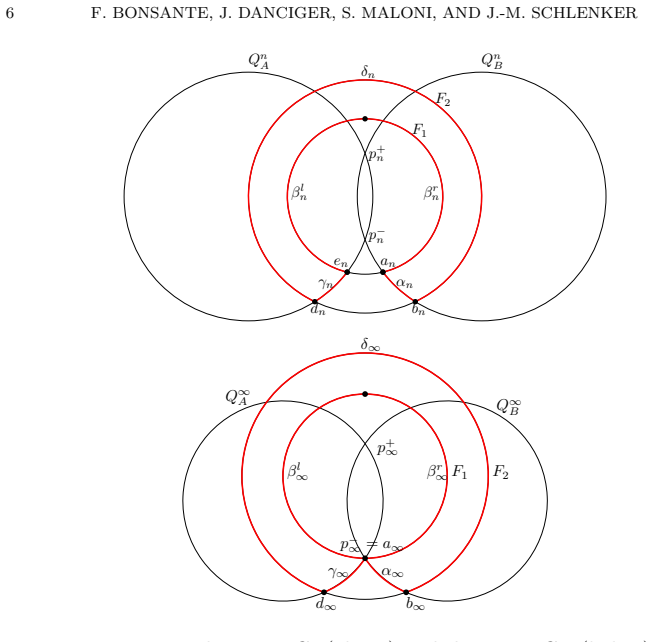
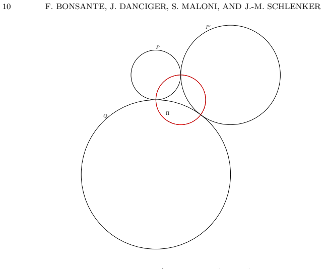
- [§3.1, Lemma 3.3] Lemma 3.3 is false as stated. In the upper half-space model, let Q={x=0} with half-space H_Q={x>0}, P={x=-1} with half-space H_P={x<-1}, and P'={x=-2} with half-space H_{P'}={x<-2}. Then P (resp. P') and Q bound disjoint half-spaces, but P∩P'=∅. Take y=(0,0,Z), x=(-1,0,Z), x'=(-2,0,Z). For Z=10 the hyperbolic distances satisfy d(x,y)<w0 and d(x',y)<w0, yet no z∈P∩P' exists. The proof's appeal to Lemma 3.2 is invalid because Lemma 3.2 assumes all three planes bound pairwise disjoint half-spaces, a hypothesis absent from Lemma 3.3. Since Corollary 3.4, Lemma 3.6, and hence Theorem 3.1 and Theorem B all rely on Lemma 3.3, this is a load-bearing gap.
- [§3.1, Lemma 3.2] The proof of Lemma 3.2 asserts that the worst case is obtained when the three lines are pairwise asymptotic and the point y is symmetrically placed, and that this reduction follows by symmetry. This reduction is not proved. Since the value w0 = cosh^{-1}(√2) is the basis for the threshold in Theorem B, a rigorous extremal argument or a reference is needed. As written, the calculation of the four congruent triangles is conditional on an unproved reduction, so Lemma 3.2 is not fully established.
- [§3.2, Proposition 3.7] In the converse direction of Proposition 3.7, the proof asserts that π+ extends continuously to the identity on C because 'π+ moves points at most by η0'. However, η0 comes from Lemma 3.8, which is proved only under the forward hypothesis that C is a quasicircle. Under the converse hypothesis, the bounded-distance estimate d(y,π+(y))≤η0 has not been established, and a quasi-isometry between ∂-C and ∂+C does not by itself guarantee that its boundary extension is the identity. The composition b+∘π+∘(b-)^(-1) therefore cannot yet be asserted to extend to the identity on C. This gap affects the conclusion that C is the image of RP^1 under a quasiconformal map and needs to be repaired, for example by proving from the quasi-isometry condition that π+ is asymptotically the identity near C.
minor comments (4)
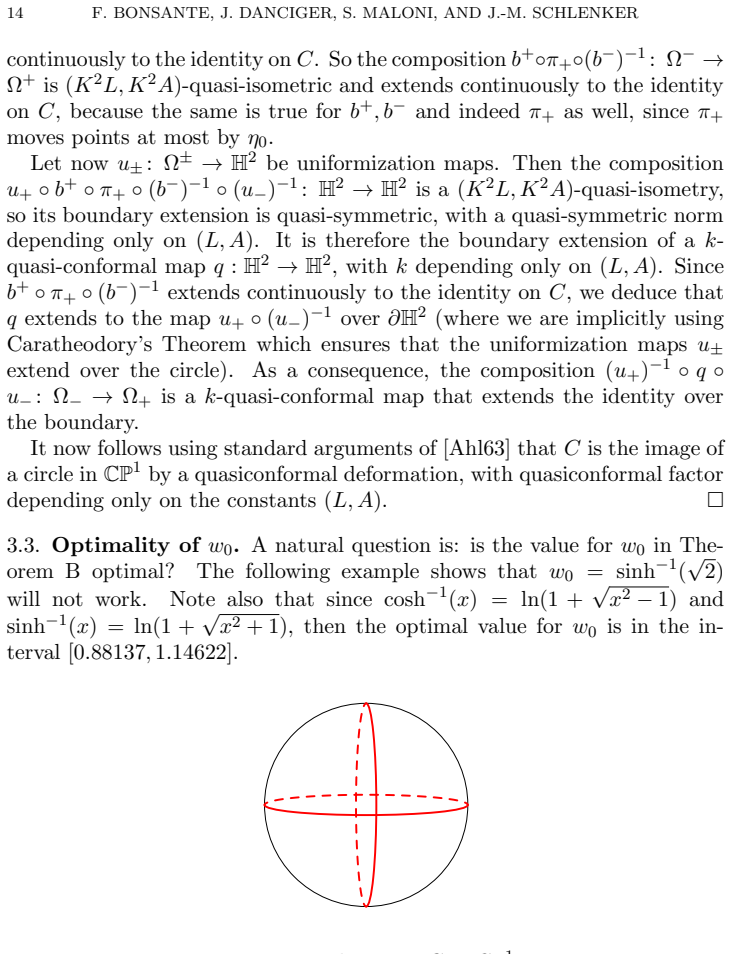
- [§3.3, Proposition 3.9] The notation is confusing because w0 was defined as cosh^{-1}(√2) at the start of Section 3, while the example in Proposition 3.9 concerns sinh^{-1}(√2). Please state explicitly that the example gives an upper bound on the optimal threshold, while Theorem B provides a lower bound.
- [§2.2, Proposition 2.4] In the proof of Proposition 2.4, the planes P^+ and P^- are introduced with boundaries in U^+ and U^-, but the sign convention is not defined. The inequality d(x_n,∂+CH(C_n)) = d(x̄,g_n(∂+CH(C_n))) < d(x̄,P^+) should be expanded, since it implicitly uses the fact that projection onto a convex set is distance-decreasing and that the chosen support planes separate the relevant regions.
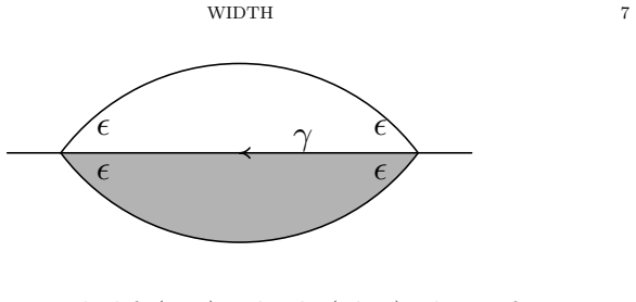
- [§2.2.1, Claim 2.6] Claim 2.6 is presented as evident from Figure 2. A short proof or a more precise statement of which complementary regions are involved would improve the exposition and make the verification of the hypotheses of Proposition 2.4 easier to check.
- [§3.2, Lemma 3.8] In the proof of Lemma 3.8, the phrase 'the path metric on f(Σ_r) is L-bilipschitz to the path metric on Σ_r' should be stated more carefully as 'L-bilipschitz to the induced path metric on Σ_r', and the subsequent 'cosh(r)-bilipschitz embedded copy of H^2' should clarify the comparison between the induced path metric on Σ_r and the hyperbolic metric on H^2. There are also minor typos such as 'equiped' in the proof of Proposition 3.7.
Circularity Check
No circularity: the width invariant is new and Theorems A–C are derived from explicit geometric estimates; self-citations are motivational.
full rationale
The paper's central claims are not obtained by fitting or by importing its own conclusions. The width w(C) and boundary width w∂(C) are new definitions, and the theorems are proved directly: Theorem A uses the explicit sequence of curves and Propositions 2.4 and 2.8; Theorem B/3.1 follows from Lemmas 3.2, 3.3, Corollary 3.4, Lemma 3.6, and Theorem C; Theorem C is proved using external results (Ahlfors, Sullivan/EM86, Tukia–Väisälä) rather than the authors' prior work. The self-citations [BS10] and [BDMS19] set up an analogy or mention an AdS counterpart, but the hyperbolic results are not reduced to those papers. No parameter is fitted to a subset of data and then renamed as a prediction. The unproved "worst case" reduction in Lemma 3.2 and the possible failure of Lemma 3.3 are mathematical correctness risks, not circularity, since a false lemma would invalidate the proof rather than make the conclusion an input.
Assumptions & free parameters
assumptions (6)
- standard math Existence and two-boundary structure of the hyperbolic convex hull of a Jordan curve in CP1
- standard math Ahlfors bounded turning criterion for quasicircles
- standard math Compactness of uniform quasicircles
- standard math Sullivan and Epstein-Marden bilipschitz comparison between the boundary of the convex hull and the conformal boundary
- standard math Tukia-Vaisala extension of quasiconformal maps to bilipschitz maps of H3
- standard math Ahlfors-Bers simultaneous uniformization and Kerckhoff-Thurston Dehn filling
Cite this review
Pith. "Pith review of Quasicircles and width of Jordan curves in $\mathbb{CP}^1$." pith.science (2026). https://pith.science/paper/JD33A77E
@misc{pith2026190809175,
  author       = {Pith},
  title        = {Pith review of: Quasicircles and width of Jordan curves in $\mathbbCP^1$},
  year         = {2026},
  howpublished = {\url{https://pith.science/paper/JD33A77E}},
  note         = {Machine review of arXiv:1908.09175}
}
abstract
We study a notion of "width" for Jordan curves in $\mathbb{CP}^1$, paying special attention to the class of quasicircles. The width of a Jordan curve is defined in terms of the geometry of its convex hull in hyperbolic three-space. A similar invariant in the setting of anti de Sitter geometry was used by Bonsante-Schlenker to characterize quasicircles amongst a larger class of Jordan curves in the boundary of anti de Sitter space. By contrast to the AdS setting, we show that there are Jordan curves of bounded width which fail to be quasicircles. However, we show that Jordan curves with small width are quasicircles.
Figures

Figures from the paper (7 more)




Reference graph
Works this paper leans on
-
[1]
Ahlfors, Quasiconformal reflections, Acta Math
Lars V. Ahlfors, Quasiconformal reflections, Acta Math. 109 (1963), 291--301. 0154978
work page 1963
-
[2]
L. V. Ahlfors, Lectures on quasiconformal mappings, D. Van Nostrand Co., Inc., Toronto, Ont.-New York-London, 1966, Manuscript prepared with the assistance of Clifford J. Earle, Jr. Van Nostrand Mathematical Studies, No. 10
work page 1966
-
[3]
Ahlfors, The structure of a finitely generated kleinian group, Acta Math
Lars V. Ahlfors, The structure of a finitely generated kleinian group, Acta Math. 122 (1969), 1--17
work page 1969
-
[4]
Anderson, Complete minimal hypersurfaces in hyperbolic n -manifolds , Comment
Michael T. Anderson, Complete minimal hypersurfaces in hyperbolic n -manifolds , Comment. Math. Helv. 58 (1983), no. 2, 264--290. 705537 (85e:53076)
work page 1983
-
[5]
Francesco Bonsante, Jeffrey Danciger, Sara Maloni, and Jean-Marc Schlenker, The induced metric on the boundary of the convex hull of a quasicircle in hyperbolic and anti de sitter geometry, arXiv preprint arXiv:1902.04027 (2019)
work page Pith review arXiv 2019
-
[6]
Lipman Bers, Simultaneous uniformization, Bull. Amer. Math. Soc. 66 (1960), 94--97. 0111834
work page 1960
-
[7]
Francesco Bonsante and Jean-Marc Schlenker, Maximal surfaces and the universal T eichm\"uller space , Invent. Math. 182 (2010), no. 2, 279--333. 2729269
work page 2010
-
[8]
D. B. A. Epstein and A. Marden, Convex hulls in hyperbolic spaces, a theorem of Sullivan , and measured pleated surfaces , Analytical and geometric aspects of hyperbolic space (D. B. A. Epstein, ed.), L.M.S. Lecture Note Series, vol. 111, Cambridge University Press, 1986
work page 1986
Show all 14 references
-
[9]
Epstein, The hyperbolic G auss map and quasiconformal reflections , J
Charles L. Epstein, The hyperbolic G auss map and quasiconformal reflections , J. Reine Angew. Math. 372 (1986), 96--135. 863521 (88b:30029)
1986
-
[10]
Kerckhoff and William P
Steven P. Kerckhoff and William P. Thurston, Noncontinuity of the action of the modular group at B ers' boundary of T eichm\" u ller space , Invent. Math. 100 (1990), no. 1, 25--47. 1037141
1990
-
[11]
Lehto and K
O. Lehto and K. I. Virtanen, Quasiconformal mappings in the plane, second ed., Springer-Verlag, New York-Heidelberg, 1973, Translated from the German by K. W. Lucas, Die Grundlehren der mathematischen Wissenschaften, Band 126. 0344463
1973
-
[12]
Andrea Seppi, Minimal discs in hyperbolic space bounded by a quasicircle at infinity, Comment. Math. Helv. 91 (2016), no. 4, 807--839. 3566524
2016
-
[13]
1979/80, Lecture Notes in Math., vol
Dennis Sullivan, Travaux de T hurston sur les groupes quasi-fuchsiens et les vari\'et\'es hyperboliques de dimension 3 \ fibr\'ees sur S^ 1 , Bourbaki S eminar, V ol. 1979/80, Lecture Notes in Math., vol. 842, Springer, Berlin-New York, 1981, pp. 196--214. 636524
1979
-
[14]
a is\" a l\
P. Tukia and J. V\" a is\" a l\" a , Quasiconformal extension from dimension n to n+1 , Ann. of Math. (2) 115 (1982), no. 2, 331--348. 647809
1982
Reviewed August 14, 2026 · model on record in the stance chip above.
Discussion (0). Continue with ORCID to comment.