REVIEW 4 major objections 5 minor 40 references
An Investigation into the Variability of Luminous Blue Variable Stars with TESS
T0 review · 4 major / 5 minor · reviewed 2026-08-10 · deepseek-v4-flash
Pith's one-line read LBV microvariability shows no link to temperature, luminosity, or mass loss.
desk verdict Useful new LBV dataset, but the central null result is under-analyzed and possibly biased by heterogeneous TESS baselines. read the letter →
The pith
A machine-rendered reading of the paper's core claim, the machinery that carries it, and where it could break.
The reading
What carries the argument
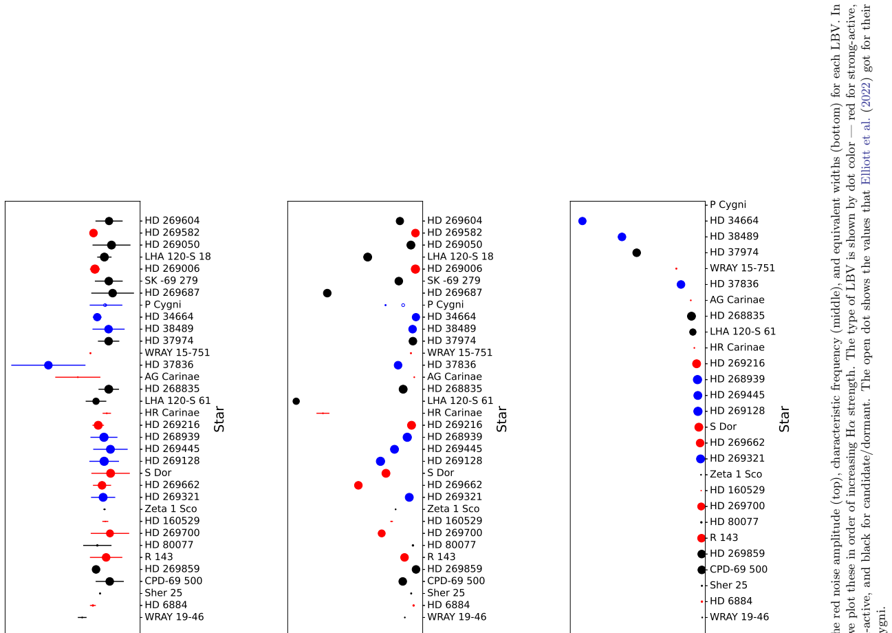
The central object is the Harvey-style semi-Lorentzian fit to the amplitude spectrum, $\alpha_\nu = \alpha_0 / (1 + (\nu/\nu_\mathrm{char})^\gamma) + C_w$, where $\alpha_0$ is the zero-frequency red noise amplitude, $\nu_\mathrm{char}$ is the characteristic frequency, $\gamma$ is the logarithmic slope, and $C_w$ is white noise. The light curves were produced from TESS full-frame images with the eleanor package, Fourier transformed with Period04, and the parameters were estimated with lmfit nonlinear regression followed by an MCMC sampler (emcee). This machinery converts each star's time series into three numbers that can be compared across a heterogeneous sample, and it is what allows the paper to test whether variability properties track stellar parameters.
What would settle it
Recompute $\alpha_0$ and $\nu_\mathrm{char}$ for the same 37 stars using a gap-aware method such as Lomb-Scargle periodograms with window-function correction, or by injecting synthetic gaps into continuous light curves; if the fitted parameters shift systematically with the number of TESS sectors or with gap structure, the reported absence of correlation could be an artifact of the sampling, not a property of the stars.
Extended reading notes
Core claim
The paper claims that the Fourier parameters of LBV light curves, specifically the red noise amplitude $\alpha_0$, the characteristic frequency $\nu_\mathrm{char}$, and the logarithmic slope $\gamma$, show no correlation with H-$\alpha$ strength, B-V color, or average g-magnitude. This absence of correlation holds for a sample spanning Galactic, LMC, and SMC LBVs and candidate LBVs, with strong-active, weak-active, and dormant classifications interleaved without any systematic pattern. The authors interpret this as confirmation that the short-term microvariations of LBVs behave like the $\alpha$ Cygni variability of hot supergiants, and they speculate that the long and short S Doradus cycles may be extensions of the same mechanism rather than a distinct phenomenon.
Load-bearing premise
The analysis treats Fourier parameters derived from light curves with very different lengths, gaps, and cadences as directly comparable, even though the software used does not account for gaps in the time series.
Editorial extensions
If this is right
- If the absence of correlation is real, the short-term variability of LBVs does not depend on temperature, luminosity, or mass-loss rate, so those parameters cannot be used to predict how an LBV will flicker.
- The lack of a clear boundary between strong-active, weak-active, and dormant/candidate LBVs suggests that these categories may reflect observing epoch and long-term phase rather than intrinsic differences in the microvariability mechanism.
- The interpretation that LBVs are an extension of alpha Cygni supergiants implies that the same driving mechanism, whether internal gravity waves or sub-surface convection, could operate across the entire upper H-R diagram.
- It follows from the paper's speculation that the long and short S Doradus cycles might be the same stochastic process seen on longer timescales, which would weaken the case for a distinct LBV variability criterion.
- If the classification were simplified, future surveys could identify LBV-like stars by their position in the H-R diagram and their stochastic variability properties rather than by requiring observed eruptions.
Reading between the lines
- A testable extension would be to compare the fitted Fourier parameters of LBVs with those of non-LBV B-type and A-type supergiants in the same TESS fields, matched in luminosity and temperature, to see whether the distributions overlap completely.
- Because the sample mixes very different time baselines and cadences, a gap-aware reanalysis with Lomb-Scargle periodograms or a window-function-corrected Fourier fit could reveal whether the reported null result is robust; this is an inference of the editor, not a claim of the paper.
- If the extension hypothesis is right, then long-baseline monitoring of LBVs should show that their S Doradus cycles have the same Fourier shape as their microvariations, just at lower frequencies, which future decade-long TESS or ASAS-SN datasets could test.
- The paper leaves open whether the red noise arises from surface convection zones or from internal gravity waves; comparing the phase behavior of photometric and spectroscopic variations for the same stars would help separate these two mechanisms.
Editorial analysis
A structured set of objections, weighed in public.
Referee Report
Summary. The paper presents a Fourier analysis of TESS light curves for 37 luminous blue variables (LBVs) and candidates drawn from the Richardson & Mehner (2018) census. Using the Harvey-style model of Eq. (1), the authors fit the amplitude spectrum of each star to obtain a red-noise amplitude alpha0, a characteristic frequency nu_char, a slope gamma, and a white-noise term Cw (Table 2). They then compare these Fourier parameters with H-alpha equivalent widths, B-V colors, and apparent g-band magnitudes (Figs. 4-7), concluding that none of the parameters correlate with these stellar properties. On this basis they argue that LBV microvariability is an extension of alpha Cygni variability in hot supergiants rather than a distinct class property, and that the LBV classification may not require a variability criterion.
Significance. If the null result is robust, the paper makes a useful observational contribution: it is the first systematic TESS-based Fourier characterization of a sample spanning Galactic, LMC, and SMC LBVs and candidates, more than tripling the sample of Nazé et al. (2021). The comparative light-curve extraction that preserves long-term S Dor-type variability, the validation against the independent BRITE analysis of P Cygni (Elliott et al. 2022), and the public availability of fit parameters in Table 2 are strengths. However, the central claim is a null result, so it stands or falls on whether the measured Fourier parameters are genuinely comparable across a sample that is extremely heterogeneous in time baseline, gap structure, and cadence, and on whether the absence of correlation is established quantitatively rather than by visual inspection. As presented, the analysis does not yet support the strength of the conclusions drawn.
major comments (4)
- [Section 4 and Figs. 4-7] The central claim of no correlation between Fourier parameters and H-alpha strength, B-V, or g-magnitude is based on visual inspection and unquantified curve fitting. No correlation coefficients, significance levels, or confidence intervals on the absence of trends are reported. For a null result that is the main finding, the paper should provide quantitative measures (e.g., Spearman or Pearson r with uncertainties from the MCMC posteriors, or an upper limit on any possible trend) to support 'confirm the absence of correlation' in the abstract.
- [Section 3 and Table 1] The intercomparability of Fourier parameters across the sample is load-bearing and is asserted rather than tested. Table 1 shows Galactic stars observed in 1-4 TESS sectors and LMC stars in 19-25 sectors, with cadence changing from 30-minute to 10-minute in years 3-4. The frequency resolution for a 1-month baseline is about 0.03 d^-1, while many fitted values of nu_char in Table 2 are below this (e.g., HD 269859 at 0.0013 d^-1, HD 269582 at 0.0027 d^-1, HD 269006 at 0.0028 d^-1, HD 34664 at 0.0015 d^-1). The paper's statement in Section 3 that 'period04 does not handle gaps in the time-series, which does provide some issues with our Fourier properties, but these Fourier properties should be intercomparable' is not sufficient. A matched-baseline test (e.g., fitting only the first four sectors of the LMC stars) or an explicit window-function analysis is needed to rule out the possibility that the apparent absence of correlation is a sampling artifact.
- [Table 2] Several of the Harvey-model fits are unphysical and appear to drive the dynamic range in the correlation plots. For example, HD 37836 has alpha0 = 1.31e6 +/- 1.9e3 ppt and Cw = 5603 +/- 34 ppt, and AG Carinae has alpha0 = 3264 +/- 99 ppt; these values are many orders of magnitude larger than typical red-noise amplitudes for the other stars and have formally tiny errors after the rescaling described in Section 3. HD 34664 has nu_char = 0.0015 +/- 0.0015 d^-1, i.e., consistent with zero. The paper should assess whether the Harvey model is appropriate for these stars, treat them as outliers or model the long-term S Dor component separately, and show that the null result is not driven by these extreme points.
- [Table 2 and Figs. 4-6] The comparison with H-alpha strength uses only a subset of the sample, since many stars in Table 2 have no W_lambda(H-alpha) measurement (e.g., HD 269687, HD 269006, HD 269582, and others). The paper does not state how many of the 37 stars have CHIRON H-alpha data, nor how missing values are handled in the correlation plots. The absence of a trend in H-alpha should be demonstrated on the subsample with actual measurements, and the sample size should be reported.
minor comments (5)
- [Figure 7] The axis labels contain typos: 'E uivalent Widths' and 'Characteristic Fre uency' should be 'Equivalent Widths' and 'Characteristic Frequency'.
- [Table 1] The TESS sector list for HD 37974 reads '1-3, 5-6, 8-3', which is likely a typo for '8-13'.
- [Section 3] The error-rescaling formula described in the text (multiplying the emcee errors by chi2_{best fit}/(0.5*Ndata - 4)) is not standard and the factor of 0.5 is not justified; a reference or derivation would help the reader understand the reported uncertainties.
- [Abstract and Section 4] The abstract states the paper 'confirm[s] the absence of correlation,' whereas Section 4 describes 'no discernible pattern' and 'no correlation found' through visual inspection and unquantified fitting; the language in the abstract is too strong given the analysis presented.
- [Fig. 4 top panel] The y-axis label reads 'Log Amplitude (Normalized Flux)' while Table 2 lists alpha0 in ppt; the units should be made consistent or explicitly converted.
Circularity Check
No significant circularity: the reported absence of correlation is an empirical null result, not a quantity forced by the fitting procedure or by self-citation.
full rationale
The paper's derivation chain is not circular. It extracts TESS light curves, fits each with a Harvey-like red-noise model (Eq. 1: alpha_nu = alpha0 / [1 + (nu/nu_char)^gamma] + C_w), and then searches for correlations between the fitted parameters and stellar observables (H-alpha equivalent width, B-V, g-magnitude). The stellar parameters are not inputs to the Fourier fit, so a null correlation cannot be forced by construction. The authors make no prediction from fitted values; the 'absence of correlation' is an empirical result rather than a consequence of the model. Target selection uses the Richardson & Mehner (2018) catalog, a self-citation, but it only defines the sample; it does not supply the measured null result or forbid alternatives. The validation against Elliott et al. (2022), which shares authors, is a methodological check of the fitting pipeline and does not determine the correlation outcome. The admitted gap-sensitivity of period04 ('period04 does not handle gaps in the time-series, which does provide some issues with our Fourier properties, but these Fourier properties should be intercomparable for the population we are examining') is a possible systematic/validity concern, not a logical circularity: even if baseline differences bias the parameters, that is a measurement artifact, not an input-output identity. No uniqueness theorem, ansatz-by-citation, or renamed known result carries the argument. There is a separate editorial inconsistency (R81 appears in Table 2 despite being rejected in Section 3 as a binary), but it does not make the reasoning circular. Overall: no significant circularity.
Assumptions & free parameters
free parameters (4)
- alpha0 (red noise amplitude) =
per star, e.g., 4.13 ppt (S Dor) to 1.31e6 ppt (HD 37836)
- nu_char (characteristic frequency) =
per star, range 0.0013 to 0.297 d^-1
- gamma (slope) =
per star, range 0.841 to 3.85
- C_w (white noise) =
per star, range 0.028 to 5603 ppt
assumptions (6)
- domain assumption The Harvey-like function (Eq. 1) adequately describes the Fourier amplitude spectrum of all 37 LBVs.
- ad hoc to paper Fourier properties from light curves with different baselines, gaps, and cadences are intercomparable without window-function correction.
- domain assumption Fitting the Fourier amplitude, rather than power, with Eq. 1 is a valid characterization.
- domain assumption H-alpha equivalent width is a proxy for mass-loss rate.
- domain assumption For LMC stars, B-V and average g magnitude are reliable relative proxies for temperature and luminosity.
- ad hoc to paper The absence of correlation can be established by visual inspection and unquantified curve fitting.
Cite this review
Pith. "Pith review of An Investigation into the Variability of Luminous Blue Variable Stars with TESS." pith.science (2026). https://pith.science/paper/JHLLNWMM
@misc{pith2026250100240,
  author       = {Pith},
  title        = {Pith review of: An Investigation into the Variability of Luminous Blue Variable Stars with TESS},
  year         = {2026},
  howpublished = {\url{https://pith.science/paper/JHLLNWMM}},
  note         = {Machine review of arXiv:2501.00240}
}
abstract
Luminous Blue Variables (LBVs) are enigmatic, evolved, massive stars. Their variability has been observed to be episodic with large eruptions, along with variations on time-scales of days to decades. We have extracted light curves of 37 LBVs from the first four years of the TESS mission. These light curves provide two years of photometric time-series for stars in the LMC, with several months of data for Galactic or SMC targets. We analyze the Fourier properties of the stellar light curves to determine their characteristic frequencies and red noise amplitudes, comparing them to mass-loss parameters through H$\alpha$ strength, and in the case of the LMC stars, $B-V$ color and luminosity as estimated by their apparent $g$-magnitudes. We confirm the absence of correlation between any of the Fourier parameters and stellar parameters, implying that there is no trend in how these stars vary as measured with these photometric data, which may point towards these stars being an extension to the supergiant $\alpha$ Cygni variables and not a unique class of object with regards to their short-term variations.
Figures


Figures from the paper (4 more)



Reference graph
Works this paper leans on
-
[1]
Aadland, E., Massey, P., Neugent, K. F., & Drout, M. R. 2018, AJ, 156, 294, doi: 10.3847/1538-3881/aaeb96
-
[2]
Aerts, C. 2021, Reviews of Modern Physics, 93, 015001, doi: 10.1103/RevModPhys.93.015001 Astropy Collaboration, Robitaille, T. P., Tollerud, E. J., et al. 2013, A&A, 558, A33, doi: 10.1051/0004-6361/201322068 Astropy Collaboration, Price-Whelan, A. M., Sip˝ ocz, B. M. , et al. 2018, AJ, 156, 123, doi: 10.3847/1538-3881/aabc4f
-
[3]
2011, A&A, 533, A4, doi: 10.1051/0004-6361/201116949
Blomme, R., Mahy, L., Catala, C., et al. 2011, A&A, 533, A4, doi: 10.1051/0004-6361/201116949
-
[4]
Bowman, D. M. 2020, Frontiers in Astronomy and Space Sciences, 7, 70, doi: 10.3389/fspas.2020.578584 —. 2023, Ap&SS, 368, 107, doi: 10.1007/s10509-023-04262-7
arXiv 2020
-
[5]
M., Burssens, S., Sim´ on-D ´ ıaz, S., et al
Bowman, D. M., Burssens, S., Sim´ on-D ´ ıaz, S., et al. 2020, A&A, 640, A36, doi: 10.1051/0004-6361/202038224
-
[6]
M., Aerts, C., Johnston, C., et al
Bowman, D. M., Aerts, C., Johnston, C., et al. 2019a, A&A, 621, A135, doi: 10.1051/0004-6361/201833662
-
[7]
Bowman, D. M., Burssens, S., Pedersen, M. G., et al. 2019b, Nature Astronomy, 3, 760, doi: 10.1038/s41550-019-0768-1
-
[8]
Burssens, S., Sim´ on-D ´ ıaz, S., Bowman, D. M., et al. 2020, A&A, 639, A81, doi: 10.1051/0004-6361/202037700
Show all 40 references
-
[9]
2016, MNRAS, 463, 3894, doi: 10.1093/mnras/stw2253
Elias-Rosa, N., Pastorello, A., Benetti, S., et al. 2016, MNRAS, 463, 3894, doi: 10.1093/mnras/stw2253
2016 doi
-
[10]
D., Pablo, H., et al
Elliott, A., Richardson, N. D., Pablo, H., et al. 2022, MNRAS, 509, 4246, doi: 10.1093/mnras/stab3112
2022 doi
-
[11]
D., Montet, B
Feinstein, A. D., Montet, B. T., Foreman-Mackey, D., et al. 2019, PASP, 131, 094502, doi: 10.1088/1538-3873/ab291c
2019 doi
-
[12]
2019, The Journal of Open Source Software, 4, 1864, doi: 10.21105/joss.01864
Foreman-Mackey, D., Farr, W., Sinha, M., et al. 2019, The Journal of Open Source Software, 4, 1864, doi: 10.21105/joss.01864
2019 doi
- [13]
-
[14]
1985, in ESA Special Publication, Vol
Harvey, J. 1985, in ESA Special Publication, Vol. 235, Future Missions in Solar, Heliospheric & Space Plasma Physics, ed. E. Rolfe & B. Battrick, 199
1985
-
[15]
M., & Davidson, K
Humphreys, R. M., & Davidson, K. 1979, ApJ, 232, 409, doi: 10.1086/157301 —. 1984, Science, 223, 243, doi: 10.1126/science.223.4633.243 —. 1994, PASP, 106, 1025, doi: 10.1086/133478
1979 doi
-
[16]
M., Weis, K., Davidson, K., & Gordon, M
Humphreys, R. M., Weis, K., Davidson, K., & Gordon, M. S. 2016, ApJ, 825, 64, doi: 10.3847/0004-637X/825/1/64
2016 doi
-
[17]
2018, Nature, 561, 498, doi: 10.1038/s41586-018-0525-0
Jiang, Y.-F., Cantiello, M., Bildsten, L., et al. 2018, Nature, 561, 498, doi: 10.1038/s41586-018-0525-0
2018 doi
-
[18]
2014, A&A, 570, A41, doi: 10.1051/0004-6361/201424313
Kallinger, T., De Ridder, J., Hekker, S., et al. 2014, A&A, 570, A41, doi: 10.1051/0004-6361/201424313
2014 doi
-
[19]
J., et al
Koenigsberger, G., Georgiev, L., Hillier, D. J., et al. 2010 , AJ, 139, 2600, doi: 10.1088/0004-6256/139/6/2600
2010 doi
-
[20]
J., et al
Koenigsberger, G., Morrell, N., Hillier, D. J., et al. 2014, AJ, 148, 62, doi: 10.1088/0004-6256/148/4/62
2014 doi
-
[21]
Spoon, H. W. W. 1998, A&A, 335, 605
1998
-
[22]
Lamers, H. J. G. L. M., & Fitzpatrick, E. L. 1988, ApJ, 324, 279, doi: 10.1086/165894
1988 doi
-
[23]
2005, Communications in Asteroseismology, 146, 53, doi: 10.1553/cia146s53
Lenz, P., & Breger, M. 2005, Communications in Asteroseismology, 146, 53, doi: 10.1553/cia146s53
2005 doi
-
[24]
2022, A&A, 657, A4, doi: 10.1051/0004-6361/202040062
Mahy, L., Lanthermann, C., Hutsem´ ekers, D., et al. 2022, A&A, 657, A4, doi: 10.1051/0004-6361/202040062
2022 doi
-
[25]
C., Smith, N., Filippenko, A
Mauerhan, J. C., Smith, N., Filippenko, A. V., et al. 2013, MNRAS, 430, 1801, doi: 10.1093/mnras/stt009 Naz´ e, Y., Rauw, G., & Gosset, E. 2021, MNRAS, 502, 5038, doi: 10.1093/mnras/stab133
2013 doi
-
[26]
D., & Gies, D
Richardson, N. D., & Gies, D. R. 2010, The Astronomer’s Telegram, 2560, 1
2010
-
[27]
D., Gies, D
Richardson, N. D., Gies, D. R., & Williams, S. J. 2011a, AJ, 142, 201, doi: 10.1088/0004-6256/142/6/201
-
[28]
D., & Mehner, A
Richardson, N. D., & Mehner, A. 2018, Research Notes of the American Astronomical Society, 2, 121, doi: 10.3847/2515-5172/aad1f3
2018 doi
-
[29]
D., Morrison, N
Richardson, N. D., Morrison, N. D., Gies, D. R., et al. 2011b, AJ, 141, 120, doi: 10.1088/0004-6256/141/4/120
-
[30]
Adelman, S. J. 2011c, AJ, 141, 17, doi: 10.1088/0004-6256/141/1/17
-
[31]
D., Schaefer, G
Richardson, N. D., Schaefer, G. H., Gies, D. R., et al. 2013, ApJ, 769, 118, doi: 10.1088/0004-637X/769/2/118
2013 doi
-
[32]
D., Pablo, H., Sterken, C., et al
Richardson, N. D., Pablo, H., Sterken, C., et al. 2018, MNRAS, 475, 5417, doi: 10.1093/mnras/sty157
2018 doi
-
[33]
R., Winn, J
Ricker, G. R., Winn, J. N., Vanderspek, R., et al. 2015, Journal of Astronomical Telescopes, Instruments, and Systems, 1, 014003, doi: 10.1117/1.JATIS.1.1.014003
2015 doi
-
[34]
E., de Koter, A., et al
Sana, H., de Mink, S. E., de Koter, A., et al. 2012, Science, 337, 444, doi: 10.1126/science.1223344 16
2012 doi
-
[35]
J., Prieto, J
Shappee, B. J., Prieto, J. L., Grupe, D., et al. 2014, ApJ, 788, 48, doi: 10.1088/0004-637X/788/1/48
2014 doi
-
[36]
Filippenko, A. V. 2011, MNRAS, 415, 773, doi: 10.1111/j.1365-2966.2011.18763.x
2011
-
[37]
2015, MNRAS, 447, 598, doi: 10.1093/mnras/stu2430
Smith, N., & Tombleson, R. 2015, MNRAS, 447, 598, doi: 10.1093/mnras/stu2430
2015 doi
-
[38]
1991, A&A, 247, 383
Sterken, C., Gosset, E., Juttner, A., et al. 1991, A&A, 247, 383
1991
-
[39]
A., Bonati, M., et al
Tokovinin, A., Fischer, D. A., Bonati, M., et al. 2013, PASP, 125, 1336, doi: 10.1086/674012
2013 doi
-
[40]
2002, A&A, 389, 931, doi: 10.1051/0004-6361:20020682 van Genderen, A
Tubbesing, S., Kaufer, A., Stahl, O., et al. 2002, A&A, 389, 931, doi: 10.1051/0004-6361:20020682 van Genderen, A. M. 2001, A&A, 366, 508, doi: 10.1051/0004-6361:20000022 van Genderen, A. M., de Groot, M., & Sterken, C. 1997, A&AS, 124, 517, doi: 10.1051/aas:1997204
2002 doi
Reviewed August 10, 2026 · model on record in the stance chip above.
Discussion (0). Continue with ORCID to comment.