REVIEW 3 major objections 5 minor 33 references
Using Neural Networks to Automate the Identification of Brightest Cluster Galaxies in Large Surveys
T0 review · 3 major / 5 minor · reviewed 2026-08-09 · deepseek-v4-flash
Pith's one-line read A neural network trained on simulated galaxy clusters can locate the brightest cluster galaxy (BCG) directly from multiband images, reaching near-perfect agreement on simulated tests, strong agreement on bright real clusters, and moderate…
desk verdict Honest proof-of-concept for image-only BCG finding; the WHL12 ground-truth caveat is real but acknowledged, and the method deserves refereeing. read the letter →
The pith
A machine-rendered reading of the paper's core claim, the machinery that carries it, and where it could break.
The reading
What carries the argument
The central object is the ResNet18 convolutional network used as a position regressor: it consumes a five-channel (SDSS u,g,r,i,z) image of a 1 Mpc region around a cluster and returns a predicted (x,y) centroid for the BCG. Training images are deliberately off-centered with a Gaussian offset of 150 kpc standard deviation so the model learns to prefer central galaxies while tolerating the offsets between BCGs and cluster centers defined by other techniques. Accuracy is measured by R² on the x- and y-coordinates and by the fraction of predictions within 25 kpc of the truth.
What would settle it
Take a sample of SDSS clusters with r_BCG>16.5, obtain independent BCG positions from deep, high-resolution imaging or from a catalog using a different definition such as redMaPPer or X-ray peaks, and measure the network's offsets against those labels; if the network agrees no better with these independent labels than with WHL12, the accuracy drop is real, but if agreement improves, the gap is largely WHL12 label error.
Extended reading notes
Core claim
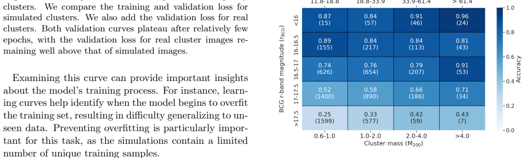
The central claim is that the BCG centroid can be regressed directly from pixel data: a ResNet18 takes a 192×192 five-band image as input and outputs the x,y position of the brightest cluster galaxy. The paper reports near-perfect performance when training and testing are both on simulations (R²≈0.94), strong performance on the brightest real clusters (R²≈0.99 for r_BCG≤16.5), and moderate performance on the full real sample (R²≈0.60), with the degradation attributed to the simulated clusters being more massive and hosting brighter BCGs than the typical real cluster. A model trained on real images transfers well to simulations, but not the reverse, suggesting the simulations cover a subset of the real diversity. The authors conclude the technique is a promising route to fast, automated BCG identification for upcoming wide surveys, with transfer learning as a pragmatic fix for dataset shift.
Load-bearing premise
The real-data evaluation takes the WHL12 catalog's BCG positions as correct, so any systematic errors in how WHL12 picks the brightest galaxy, particularly for dim or distant clusters, are counted as failures of the network rather than as label noise.
Editorial extensions
If this is right
- Simulation-trained networks can pre-publish BCG catalogs for surveys before real calibration data arrive, with the caveat that accuracy is high only when the real clusters resemble the simulated ones.
- A characteristic cut such as r_BCG ≤ 16.5 selects a regime where the network is reliable, giving a simple operational rule for users of large surveys.
- Fine-tuning with a few hundred real images corrects most of the simulation bias, so early small data releases can be leveraged to adapt the model quickly.
- The network outperforms choosing the brightest galaxy in the field, especially in the presence of foreground interlopers, and it degrades more slowly with redshift.
- Performance drops sharply beyond z≈0.6, but it is unclear whether that is an SDSS depth or resolution limit or an intrinsic limit of the approach.
Reading between the lines
- A natural extension the paper does not test is applying the same architecture to deeper, higher-resolution surveys like Euclid or Rubin using their filter sets; the pipeline is band-agnostic, so the redshift ceiling could shift upward.
- The paper's evidence that simulations form a subset of real images suggests a direct improvement: enriching simulated training sets with dimmer and less massive clusters should improve generalization to the full real sample.
- The confidence or uncertainty prediction suggested in the discussion could be implemented as a two-headed network that also outputs a variance, letting users flag low-confidence detections rather than relying on a magnitude cut.
- Since WHL12 labels are themselves derived by picking the brightest nearby galaxy, the reported accuracy on real data conflates network errors with catalog errors; a cleaner test would compare against visually verified BCGs.
Editorial analysis
A structured set of objections, weighed in public.
Referee Report
Summary. The paper proposes a neural-network method to identify brightest cluster galaxy (BCG) centroids directly from multiband photometric images, with the goal of automating BCG identification in large surveys. The authors train a ResNet18 on mock observations derived from The Three Hundred simulations, adding SDSS sky noise to improve realism, and test it on simulated images and on SDSS cluster images from the WHL12 catalog. They report R^2 ≈ 0.94 between predictions and truth on simulations, R^2 ≈ 0.60 on the full real-data test set, and R^2 ≈ 0.99 for the bright subset with r_BCG ≤ 16.5. The paper also compares transfer learning from simulations to real data, benchmarks against a SExtractor-based brightest-galaxy baseline, and studies performance as a function of redshift. The central claim is that neural networks are a promising method for automating BCG identification, especially when trained on simulations and applied to bright, low-redshift clusters.
Significance. If the central claim is supported, the method would be a practical contribution for upcoming wide-field surveys such as Euclid and Rubin/LSST, since it requires only photometric images and no per-galaxy redshift or source catalog. The paper has several strengths: the simulation test uses a cluster-level split, avoiding leakage between training and test projections; the comparison against a SExtractor brightest-galaxy baseline is a useful sanity check; and the transfer-learning experiments quantify how much real data are needed to correct simulation bias. The main weakness is that the real-data evaluation uses WHL12 catalog entries as ground truth, so the reported real-data accuracy measures agreement with a heuristic rather than independent physical truth. This issue is acknowledged in the text but not quantified, and it bears directly on the paper's headline real-data results.
major comments (3)
- [§4.3 (also §2.2, §5)] The real-data evaluation uses WHL12 catalog entries as ground truth. WHL12 defines the BCG as the brightest galaxy within a fixed distance from the cluster center, so the reported R^2 ≈ 0.60 on real data and R^2 ≈ 0.99 on the bright subset measure agreement with that heuristic, not independent physical identification. The sentence in §4.3 that dim BCGs are also challenging for WHL12 acknowledges the issue but does not quantify label noise. For the central claim that the network identifies BCGs in real surveys, the authors should validate on an independent label set (e.g., redMaPPer candidates, visual inspection, or spectroscopically confirmed members) or explicitly reframe the real-data results as emulation of the WHL12 algorithm.
- [§4.3, Figure 6] The bright-subset result R^2 ≈ 0.99 rests on only 60 test clusters, and no uncertainties or confidence intervals are reported for the R^2 or A_T statistics anywhere in the paper. With n = 60, a handful of outliers can move R^2 substantially, so the comparison among 0.94, 0.60, and 0.99 is not established. Please provide bootstrap or jackknife uncertainties for all reported R^2 and accuracy values. In addition, because the r_BCG ≤ 16.5 cut was chosen after inspecting Figure 5, either justify it a priori or confirm it on an independent held-out sample to avoid post-hoc selection inflating the apparent performance.
- [§4.6, Figure 10, and Abstract] The abstract and Section 5 state that the method performs well up to z ≈ 0.6, but the redshift test in §4.6 uses networks trained on real SDSS images, not the simulation-trained network that is the paper's main proposal. The simulation-trained model is only tested at z = 0.15–0.25. Please state explicitly which model supports the z ≈ 0.6 claim, or add a corresponding test of the simulation-trained model if that is the intended claim.
minor comments (5)
- [Abstract and §1] There are typographical errors: 'such those' should be 'such as those' in the abstract, and 'advantanges' should be 'advantages' in the introduction.
- [§3.1] The sentence 'We select a ResNet18 architecture and pass the x and y pixel values of the BCG centroid as learned parameters' is confusing; the x and y values are the network outputs, not learned parameters, and the wording should be corrected.
- [§3.2, Eq. (4)] The indicator notation '1≤ T(di)' is hard to parse; it should be typeset as an indicator function, e.g., \mathbb{1}[d_i \le T], and the definition should be stated in words as well.
- [Table 1 and §4.6] The 'Real (full redshift)' row in Table 1 uses dashes in a way that is unclear; specify the training and test sample sizes explicitly in the table or caption. The redshift experiment in §4.6 should also clarify whether the 'full redshift' training set and the test set are disjoint at the cluster level, not merely at the image level.
- [§3.1] The off-centering distribution is truncated at roughly 167 kpc because of the 1 Mpc cutout, so the model never sees BCG offsets beyond that value. If target surveys have larger BCG-to-center offsets, performance may degrade; please discuss this limitation explicitly.
Circularity Check
No circularity: the neural network predictions are evaluated against independently defined labels and no derivation reduces to its own inputs.
full rationale
This paper is an empirical machine-learning study, not a derivation chain, and its claims are not circular. The network is trained on simulated cluster images from The Three Hundred project with BCG positions defined by the simulation, and tested on held-out simulated images plus real SDSS images whose BCG labels come from the external WHL12 catalog. The reported statistics R^2 ≈ 0.94 on simulations, R^2 ≈ 0.60 on real data, and R^2 ≈ 0.99 on the bright r_BCG ≤ 16.5 subset are measured post-hoc on held-out data rather than being produced by fitting the same quantity that is later predicted. The only potentially load-bearing external input, the WHL12 BCG label, is cited as an independent catalog and the paper explicitly concedes that dim BCGs may be misidentified in that catalog, which is an honest caveat rather than a circular step. The selection of the bright subset is a soundness and generalization concern, not a circularity concern, because the model parameters and the subset definition do not depend on the evaluation labels in any way that forces the reported result. No equation is defined in terms of its own conclusion, no fitted parameter is renamed as a prediction, and no self-citation is used to justify a core premise. Verdict: no significant circularity.
Assumptions & free parameters
free parameters (4)
- offset_std_dev =
150 kpc (truncated at ~167 kpc)
- accuracy_threshold_T =
25 kpc
- bright_subset_cut =
r_BCG ≤ 16.5
- training_epochs =
100
assumptions (3)
- domain assumption The Three Hundred gizmo-simba simulations produce BCG photometry and large-scale environment representative of real SDSS clusters.
- domain assumption WHL12 BCG positions, Petrosian r_BCG, and the mass-richness scaling relation are accurate enough for ground truth and subsetting.
- ad hoc to paper The synthetic off-centering Gaussian (σ = 150 kpc, truncated at ~167 kpc) covers the real BCG offset distribution in surveys.
Cite this review
Pith. "Pith review of Using Neural Networks to Automate the Identification of Brightest Cluster Galaxies in Large Surveys." pith.science (2026). https://pith.science/paper/JTZDGAQL
@misc{pith2026250200104,
  author       = {Pith},
  title        = {Pith review of: Using Neural Networks to Automate the Identification of Brightest Cluster Galaxies in Large Surveys},
  year         = {2026},
  howpublished = {\url{https://pith.science/paper/JTZDGAQL}},
  note         = {Machine review of arXiv:2502.00104}
}
abstract
Brightest cluster galaxies (BCGs) lie deep within the largest gravitationally bound structures in existence. Though some cluster finding techniques identify the position of the BCG and use it as the cluster center, other techniques may not automatically include these coordinates. This can make studying BCGs in such surveys difficult, forcing researchers to either adopt oversimplified algorithms or perform cumbersome visual identification. For large surveys, there is a need for a fast and reliable way of obtaining BCG coordinates. We propose machine learning to accomplish this task and train a neural network to identify positions of candidate BCGs given no more information than multiband photometric images. We use both mock observations from The Three Hundred project and real ones from the Sloan Digital Sky Survey (SDSS), and we quantify the performance. Training on simulations yields a squared correlation coefficient, R$^2$, between predictions and ground truth of R$^2 \approx 0.94$ when testing on simulations, which decreases to R$^2 \approx 0.60$ when testing on real data due to discrepancies between datasets. Limiting the application of this method to real clusters more representative of the training data, such those with a BCG r-band magnitude $r_{\text{BCG}} \leq 16.5$, yields R$^2 \approx 0.99$. The method performs well up to a redshift of at least $z\approx 0.6$. We find this technique to be a promising method to automate and accelerate the identification of BCGs in large datasets.
Figures


Figures from the paper (6 more)



Reference graph
Works this paper leans on
-
[1]
2011, ApJS, 193, 29, doi: 10.1088/0067-0049/193/2/29
Aihara, H., Allende Prieto, C., An, D., et al. 2011, ApJS, 193, 29, doi: 10.1088/0067-0049/193/2/29
-
[2]
2017, MNRAS, 470, 2617, doi: 10.1093/mnras/stx721 2 https://www.the300-project.org
Alam, S., Ata, M., Bailey, S., et al. 2017, MNRAS, 470, 2617, doi: 10.1093/mnras/stx721 2 https://www.the300-project.org
-
[3]
1996, A&AS, 117, 393, doi: 10.1051/aas:1996164
Bertin, E., & Arnouts, S. 1996, A&AS, 117, 393, doi: 10.1051/aas:1996164
-
[4]
E., Stalder, B., de Haan, T., et al
Bleem, L. E., Stalder, B., de Haan, T., et al. 2015, The Astrophysical Journal Supplement Series, 216, 27, doi: 10.1088/0067-0049/216/2/27
-
[5]
Bottrell, C., Hani, M. H., Teimoorinia, H., et al. 2019, MNRAS, 490, 5390, doi: 10.1093/mnras/stz2934 13
-
[6]
Brough, S., Ahad, S. L., Bah´ e, Y. M., et al. 2024, MNRAS, 528, 771, doi: 10.1093/mnras/stad3810
-
[7]
2003, MNRAS, 344, 1000, doi: 10.1046/j.1365-8711.2003.06897.x
Bruzual, G., & Charlot, S. 2003, MNRAS, 344, 1000, doi: 10.1046/j.1365-8711.2003.06897.x
-
[8]
2003, PASP, 115, 763, doi: 10.1086/376392
Chabrier, G. 2003, PASP, 115, 763, doi: 10.1086/376392
doi:10.1086/376392 2003
Show all 33 references
-
[9]
2021, A&A, 649, A42, doi: 10.1051/0004-6361/202040245
Chu, A., Durret, F., & M´ arquez, I. 2021, A&A, 649, A42, doi: 10.1051/0004-6361/202040245
2021 doi
-
[10]
2022, Astronomy & Astrophysics, 666, A54, doi: 10.1051/0004-6361/202243504
Chu, A., Sarron, F., Durret, F., & M´ arquez, I. 2022, Astronomy & Astrophysics, 666, A54, doi: 10.1051/0004-6361/202243504
2022 doi
-
[11]
2016, Monthly Notices of the Royal Astronomical Society, 456, 2566, doi: 10.1093/mnras/stv2839
Cui, W., Power, C., Biffi, V., et al. 2016, Monthly Notices of the Royal Astronomical Society, 456, 2566, doi: 10.1093/mnras/stv2839
2016 doi
-
[12]
2018, MNRAS, 480, 2898, doi: 10.1093/mnras/sty2111
Cui, W., Knebe, A., Yepes, G., et al. 2018, MNRAS, 480, 2898, doi: 10.1093/mnras/sty2111
2018 doi
-
[13]
2022, MNRAS, 514, 977, doi: 10.1093/mnras/stac1402 De Lucia, G., & Blaizot, J
Cui, W., Dave, R., Knebe, A., et al. 2022, MNRAS, 514, 977, doi: 10.1093/mnras/stac1402 De Lucia, G., & Blaizot, J. 2007, Monthly Notices of the Royal Astronomical Society, 375, 2–14, doi: 10.1111/j.1365-2966.2006.11287.x De Propris, R., West, M. J., Andrade-Santos, F., et al....
2022
-
[14]
H., Gettings, D
Gonzalez, A. H., Gettings, D. P., Brodwin, M., et al. 2019, The Astrophysical Journal Supplement Series, 240, 33, doi: 10.3847/1538-4365/aafad2
2019 doi
-
[15]
2019, MNRAS, 483, 3545, doi: 10.1093/mnras/sty3203
Gozaliasl, G., Finoguenov, A., Tanaka, M., et al. 2019, MNRAS, 483, 3545, doi: 10.1093/mnras/sty3203
2019 doi
-
[16]
2015, Deep Residual Learning for Image Recognition
He, K., Zhang, X., Ren, S., & Sun, J. 2015, Deep Residual Learning for Image Recognition. https://arxiv.org/abs/1512.03385 Ivezi´ c,ˇZ., Kahn, S. M., Tyson, J. A., et al. 2019, ApJ, 873, 111, doi: 10.3847/1538-4357/ab042c
2015 arXiv
-
[17]
P., & Ba, J
Kingma, D. P., & Ba, J. 2017, Adam: A Method for Stochastic Optimization. https://arxiv.org/abs/1412.6980
2017 arXiv
-
[18]
2023, ApJS, 267, 41, doi: 10.3847/1538-4365/ace052
Kluge, M., & Bender, R. 2023, ApJS, 267, 41, doi: 10.3847/1538-4365/ace052
2023 doi
- [19]
-
[20]
2022, A&A, 661, A2, doi: 10.1051/0004-6361/202141120
Liu, A., Bulbul, E., Ghirardini, V., et al. 2022, A&A, 661, A2, doi: 10.1051/0004-6361/202141120
2022 doi
-
[21]
L., & Gonzalez, A
Mancone, C. L., & Gonzalez, A. H. 2012, Publications of the Astronomical Society of the Pacific, 124, 606–615, doi: 10.1086/666502
2012 doi
-
[22]
Muzzin, A., Wilson, G., Yee, H. K. C., et al. 2009, The Astrophysical Journal, 698, 1934, doi: 10.1088/0004-637X/698/2/1934
2009 doi
-
[23]
2010, in , 807–814 Planck Collaboration, Ade, P
Nair, V., & Hinton, G. 2010, in , 807–814 Planck Collaboration, Ade, P. A. R., Aghanim, N., et al. 2016, A&A, 594, A27, doi: 10.1051/0004-6361/201525823
2010 doi
-
[24]
2024, The Open Journal of Astrophysics, 7, 65, doi: 10.33232/001c.122309
Roche, C., McDonald, M., Borrow, J., et al. 2024, The Open Journal of Astrophysics, 7, 65, doi: 10.33232/001c.122309
2024 doi
-
[25]
S., Rozo, E., Busha, M
Rykoff, E. S., Rozo, E., Busha, M. T., et al. 2014, The Astrophysical Journal, 785, 104, doi: 10.1088/0004-637x/785/2/104
2014 doi
-
[26]
2023, Astronomy & Astrophysics, 671, A57, doi: 10.1051/0004-6361/202245138
Seppi, R., Comparat, J., Nandra, K., et al. 2023, Astronomy & Astrophysics, 671, A57, doi: 10.1051/0004-6361/202245138
2023 doi
-
[27]
C., Ryczanowski, D., Bianconi, M., et al
Smith, J. C., Ryczanowski, D., Bianconi, M., et al. 2023, Research Notes of the American Astronomical Society, 7, 51, doi: 10.3847/2515-5172/acc333
2023 doi
-
[28]
2022, AJ, 163, 146, doi: 10.3847/1538-3881/ac5030
Somboonpanyakul, T., McDonald, M., Noble, A., et al. 2022, AJ, 163, 146, doi: 10.3847/1538-3881/ac5030
2022 doi
-
[29]
2020, Journal of Open Source Software, 5, 2505, doi: 10.21105/joss.02505 van den Bosch, F
Tejero-Cantero, A., Boelts, J., Deistler, M., et al. 2020, Journal of Open Source Software, 5, 2505, doi: 10.21105/joss.02505 van den Bosch, F. C., Weinmann, S. M., Yang, X., et al. 2005, MNRAS, 361, 1203, doi: 10.1111/j.1365-2966.2005.09260.x
2020
-
[30]
R., Forman, W., et al
Vikhlinin, A., McNamara, B. R., Forman, W., et al. 1998, ApJ, 502, 558, doi: 10.1086/305951
1998 doi
-
[31]
L., Han, J
Wen, Z. L., Han, J. L., & Liu, F. S. 2012, The Astrophysical Journal Supplement Series, 199, 34, doi: 10.1088/0067-0049/199/2/34
2012 doi
-
[32]
Wilson, G., Muzzin, A., Yee, H. K. C., et al. 2009, ApJ, 698, 1943, doi: 10.1088/0004-637X/698/2/1943
2009 doi
-
[33]
G., Adelman, J., Anderson, John E., J., et al
York, D. G., Adelman, J., Anderson, John E., J., et al. 2000, AJ, 120, 1579, doi: 10.1086/301513
2000 doi
Reviewed August 9, 2026 · model on record in the stance chip above.
Discussion (0). Continue with ORCID to comment.