REVIEW 4 major objections 4 minor 103 references
CMB-S4: Foreground-Cleaning Pipeline Comparison for Measuring Primordial Gravitational Waves
T0 review · 4 major / 4 minor · reviewed 2026-08-08 · deepseek-v4-flash
Pith's one-line read The paper claims that three foreground-cleaning pipelines for CMB-S4 recover the tensor-to-scalar ratio with comparable precision on simple and intermediate-complexity simulated foregrounds, but that complex foregrounds produce biases at…
desk verdict A careful, transparent comparison of three foreground-cleaning approaches at CMB-S4 noise; the main claims hold for the simulated inputs, but the single-foreground-realization caveat and a misstated abstract significance need fixing. read the letter →
The pith
A machine-rendered reading of the paper's core claim, the machinery that carries it, and where it could break.
The reading
What carries the argument
The three pipelines share the linear data model $d = As + n$ but differ in priors and operational space. Pipeline A is a power-spectrum-based parametric method: it fits modified-blackbody dust and power-law synchrotron SEDs, including frequency-decorrelation parameters, to purified B-mode bandpowers via a Hamimeche-Lewis likelihood. Pipeline B is a non-parametric map-based ILC: it estimates CMB weights from a cross-frequency covariance with leave-one-mode-out masking and subtracts a simulation-based noise bias. Pipeline C is a map-based parametric method: it maximizes the profile spectral likelihood for foreground spectral parameters and then applies a least-squares estimator to reconstruct CMB and foreground maps. The lensing B-mode template, built by iterative MAP delensing of the LAT maps, is added to pipeline A as a pseudo-frequency band and cross-correlated with the cleaned maps in pipelines B and C; the extended variants marginalize over foreground residual power, using free decorrelation parameters in A, a weighted dust power template in B, and a linear combination of recovered dust and synchrotron spectra in C.
What would settle it
Take the first year of real CMB-S4 deep-patch data and run the three extended pipelines on the same maps; if the per-realization scatter in $r$ between pipelines substantially exceeds the simulation-predicted scatter from Table II, or if the recovered foreground spectral indices differ from the simulated model inputs by more than the reported uncertainties, then the simulated foregrounds are not representative and the paper's pipeline ranking would not transfer to real data.
Extended reading notes
Core claim
The paper's main result is a head-to-head comparison of three approaches in one simulation framework at CMB-S4 SAT noise levels: a parametric maximum-likelihood fit to the auto- and cross-frequency B-mode spectra, with the lensing template added as a pseudo-frequency band (pipeline A); a harmonic-space internal linear combination with mode-masked covariance estimation (pipeline B); and a map-based parametric maximum-likelihood reconstruction of CMB, dust, and synchrotron (pipeline C). Across the three validation foreground suites, unbiased $r$ is recovered for the Gaussian and amplitude-modulated models; with the Vansyngel suite all nominal pipelines show positive biases, for input $r=0$ corresponding to 1.6–1.9 $\sigma$. Adding foreground-residual marginalization brings the biases below roughly 0.1 $\sigma$, but increases $\sigma(r)$ by 15–20% for pipelines A and B and up to 160% for pipeline C; for input $r=0.003$ the detection significance becomes about 4.2 $\sigma$ (A), 3.4 $\sigma$ (B), and 1.8 $\sigma$ (C). On the PySM single-realization suites with the extended pipelines, pipeline A recovers $r$ within 1 $\sigma$ for all complexity levels, pipeline B shows a slight positive bias for non-zero $r$, and pipeline C does not recover an unbiased posterior for the most complex model.
Load-bearing premise
The load-bearing premise is that the simulated foreground suites, especially the single fixed realizations of the Vansyngel and PySM models, faithfully represent the polarized Galactic foregrounds that CMB-S4 will actually see in its deep patch; if the real sky's spectral decorrelation or spatial variability lies outside these models, the measured biases, the effectiveness of extended residual marginalization, and the pipeline ordering could all change.
Editorial extensions
If this is right
- At CMB-S4 South Pole noise levels and with Gaussian or amplitude-modulated foregrounds, all three pipelines deliver $\sigma(r) \sim 3$–$5 \times 10^{-4}$, consistent with reaching a roughly 5-sigma detection for $r=0.003$ when foregrounds are this simple.
- Nominal pipelines can be biased at 1.6–1.9 sigma on complex foregrounds such as the Vansyngel model, so a naive blind analysis could report a spurious detection or miss the true one.
- Marginalizing over foreground residuals removes the bias but degrades precision; for $r=0.003$ the achievable detection significance depends on pipeline choice: about 4.2 sigma (A), 3.4 sigma (B), and 1.8 sigma (C).
- Correlations between pipeline estimates drop on complex foregrounds, with the correlation between pipelines B and C falling as low as 0.44, so agreement between methods cannot be assumed and cross-validating independent pipelines on the same data is necessary.
- Pipeline A's stability across all foreground suites suggests the cross-spectral parametric method should be a primary anchor for CMB-S4 $r$ analyses, with map-based pipelines serving as cross-checks.
Reading between the lines
- Editorial inference: since Models 2–5 each supply only a single fixed foreground realization, the bias and sensitivity ranking carries no foreground sample variance; real skies with different spatial realizations could reorder the pipelines, so repeat-foreground simulation suites should be used before final pipeline selection.
- Editorial inference: the failures of pipelines B and C on high-complexity models point to spatially adaptive cleaning as the natural next step; testing needlet ILC or multi-patch parametric cleaning on the same suites would clarify whether the gap is fundamental or implementation-specific.
- Editorial inference: the paper's delensing step lowers $\sigma(r)$ by roughly a factor of 6–10, so if the real lensing-template noise cannot be characterized as accurately as in simulations, the quoted 2–4 sigma detection significance may be optimistic.
- Editorial inference: a direct testable extension is to apply the three extended pipelines to one realistic multi-frequency sky with an injected $r=0.003$ signal; if the recovered $r$ posteriors do not overlap, the residual-marginalization models are missing something.
Editorial analysis
A structured set of objections, weighed in public.
Referee Report
Summary. The paper compares three foreground-cleaning pipelines—a parametric cross-spectrum method (Pipeline A), a harmonic-space ILC (Pipeline B), and a map-based parametric maximum-likelihood method (Pipeline C)—for estimating the tensor-to-scalar ratio r from simulated CMB-S4 South Pole Deep Patch SAT maps. It validates the pipelines on three foreground suites (Gaussian, amplitude-modulated, Vansyngel) using 500 simulations per suite, applies a LAT-based iterative internal delensing step, and then tests the pipelines on PySM Models 3–5 with single realizations and MCMC posteriors. The central result is that nominal pipelines give comparable σ(r) ≈ 3–5×10^-4 and unbiased r for simple/intermediate foregrounds, but 1–2σ biases appear for the more complex Vansyngel model; extended pipelines that marginalize residual foregrounds reduce the biases to <0.1σ at the cost of increased σ(r), yielding a pipeline-dependent detection significance of 2–4σ for r=0.003, with Pipeline A showing the best stability and overall performance.
Significance. If the results hold, this is a valuable cross-validation of component-separation methods at the very low noise levels planned for CMB-S4. The paper benefits from 500 simulations per foreground suite, shared input skies across pipelines, inter-pipeline correlation analysis, and a validated iterative delensing step. It also makes good use of public tools (PySM, NaMaster, S2Hat, Cobaya) and gives a clear conceptual framing of the three methods. The main caveats—the single-realization nature of the Vansyngel and PySM foregrounds and the absence of a foreground-sample-variance term in the error budget—are acknowledged by the authors but not quantified; the abstract's 2–4σ detection range also omits the 1.8σ result of extended Pipeline C. These issues are correctable and do not invalidate the central comparison, but they need to be addressed before the headline claims can be taken at face value.
major comments (4)
- [§IV B 3–4, §VII C, Table II] Models 2–5 each provide only a single fixed foreground realization, so the extended-pipeline bias statements (<0.1σ) and the pipeline ranking are conditional on one foreground draw. No foreground-to-foreground scatter enters the error budget or the pipeline comparison, yet the paper claims that contamination is reduced 'to within statistical uncertainties.' The single-realization limitation is acknowledged in the text, but its impact on the headline comparison is not quantified. The claims should be reworded as conditional on the specific realizations used, and the absence of foreground sample variance should be stated as a limitation of the comparison rather than only a property of the foreground models.
- [§VII C, Table II, Abstract] The abstract and conclusions quote a detection significance of 2–4σ for r=0.003, but the extended Pipeline C result in Table II is r = 3.09 ± 1.75 (×10^-3), i.e. about 1.8σ. This is outside the quoted range. The text should either restrict the 2–4σ statement to Pipelines A and B or report the full pipeline-dependent range, including the 1.8σ result of Pipeline C.
- [§VI, Eqs. (6.1)–(6.2), §VII C] The extended pipelines reduce bias by adding fitted residual parameters whose templates are constructed from the same foreground model/realization used to generate the data: Eq. (6.1) uses the Pipeline A foreground model, and Eq. (6.2) uses Pipeline C's component-separated dust and synchrotron maps. The exercise therefore cannot distinguish a marginalization that generically absorbs residual foreground power from one that overfits the specific spectral/spatial structure of a single realization. This matters for the general claim of unbiased recovery: in Table III, Model 5, extended Pipelines B and C exclude the input r=0.003 at 95% credibility, showing that the 'within statistical uncertainties' statement is too strong.
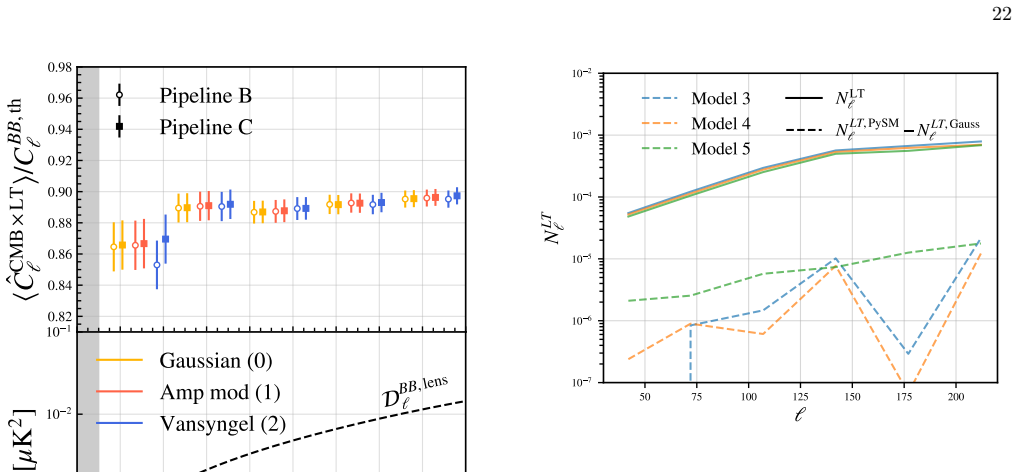
- [§V, App. B] The delensing validation uses the true foreground templates to estimate the lensing-template noise N_LT, which is not available in real data. The Gaussian-foreground test in App. B quantifies the difference in N_LT but does not propagate that difference to the r posterior. The paper asserts that the impact on r is negligible, but this is not demonstrated. The r results after delensing therefore remain dependent on perfect foreground knowledge, and this caveat should be stated more prominently.
minor comments (4)
- [§VII C] In the paragraph on the relative impact of dust and synchrotron, 'Model 3' appears to be a typo for 'Model 2': the quoted bias of 0.56 ± 0.35 matches the Vansyngel model in Table II, and the surrounding text discusses Models 0–2.
- [Fig. 3 caption] The word 'embeded' should be 'embedded' in the caption.
- [§V] The word 'appoach' should be 'approach' in the sentence describing the alternative to using the fiducial foreground simulations in constructing N_LT.
- [Table III] The header says '2σ credibility intervals' but the quoted intervals are 95% credibility intervals; please make the notation consistent (95% credibility corresponds to approximately 1.96σ for a Gaussian posterior).
Circularity Check
No significant circularity: the pipeline comparison is benchmarked against known simulation inputs, and the extended-pipeline bias removal is a model-flexibility effect, not a self-referential prediction.
full rationale
The central derivation chain is a simulation-based benchmark. Pipelines A, B, and C are applied to maps generated from known input values of r (0 and 0.003) and known foreground models, and the reported bias and sigma(r) values are measured against those inputs, so the headline comparison is externally grounded. The extended pipelines do add nuisance parameters (Delta'_d/Delta'_s in Pipeline A; A_d/alpha_d in Eq. 6.1; A'_d/A'_s in Eq. 6.2) that are fit to the same Model 2 data, and the paper explicitly presents the post-extension unbiased recovery as a demonstration of marginalization, not as a prediction independent of those fits. Fitting residual degrees of freedom to absorb residual foreground power is a standard inference step, not a circular reduction of r to the inputs; no equation in the paper defines r in terms of the fitted parameters by construction. The single-realization limitation for Models 2-5 (Sec. IV B 3 and IV B 4) removes foreground sample variance from the error budget and is acknowledged by the authors: 'Note that for this specific foreground model there is only one realization such that every map in our simulation suite contains the exact same foreground component,' and 'As with the Vansyngel model (Model 2), we have only a single realization of the foreground emission for each of Models 3, 4, and 5.' Similarly, the lensing-template noise for Models 2-5 is estimated from the same fixed foregrounds (Sec. V), so foreground leakage into the template is exactly captured by N_LT; the authors flag that this is an idealization not achievable in real data. These are robustness limitations, not circularity. Self-citations to Ref. [15] and Ref. [88] supply the noise/delensing infrastructure but are not the load-bearing argument for the pipeline comparison, which is independently evaluated against the simulated inputs.
Assumptions & free parameters
free parameters (10)
- beta_d (dust spectral index) =
Input 1.6 in Model 0; fitted per realization in Pipelines A and C
- beta_s (synchrotron spectral index) =
Input -3.1 in Model 0; fitted in Pipelines A and C
- A_d (dust amplitude at ell=80) =
Input 4.25 microK^2 in Model 0; fitted in Pipeline A
- A_s (synchrotron amplitude at ell=80) =
Input 3.8 microK^2 in Model 0; fitted in Pipeline A
- alpha_d (dust spatial spectral slope) =
Input -0.4; fitted in Pipeline A
- alpha_s (synchrotron spatial spectral slope) =
Input -0.6; fitted in Pipeline A
- epsilon (dust-synchrotron correlation) =
Varied; no fiducial quoted
- Delta'_d and Delta'_s (frequency decorrelation) =
Varied in extended Pipeline A; fixed in nominal
- A'_d and A'_s (residual amplitudes in Pipeline C) =
Varied per realization
- Ad and alpha_d in Pipeline B residual model =
Varied
assumptions (6)
- domain assumption The linear data model d = A s + n with Gaussian noise and known noise covariance N is valid for the SAT maps.
- domain assumption Galactic dust follows a modified blackbody SED with fixed T_d = 19.6 K and synchrotron follows a power-law SED.
- domain assumption Foreground BB power spectra are power laws in ell with amplitude, slope, and dust/synchrotron correlation modeled by Eqs. 3.17-3.19.
- domain assumption The ILC method may reconstruct the CMB from a linear combination of frequency maps assuming a known, frequency-independent CMB spectrum and statistical independence from contaminants.
- domain assumption The lensing template B_LT is a noisy, isotropically filtered version of the true lensing B-mode, with additive noise N_LT (Eq. 5.2).
- domain assumption The simulated foreground suites (Models 0-5) are representative of the real polarized foreground sky in the CMB-S4 patch; Models 2-5 provide only one foreground realization.
Cite this review
Pith. "Pith review of CMB-S4: Foreground-Cleaning Pipeline Comparison for Measuring Primordial Gravitational Waves." pith.science (2026). https://pith.science/paper/JWP6J34G
@misc{pith2026250204300,
  author       = {Pith},
  title        = {Pith review of: CMB-S4: Foreground-Cleaning Pipeline Comparison for Measuring Primordial Gravitational Waves},
  year         = {2026},
  howpublished = {\url{https://pith.science/paper/JWP6J34G}},
  note         = {Machine review of arXiv:2502.04300}
}
abstract
We compare multiple foreground-cleaning pipelines for estimating the tensor-to-scalar ratio, $r$, using simulated maps of the planned CMB-S4 experiment within the context of the South Pole Deep Patch. To evaluate robustness, we analyze bias and uncertainty on $r$ across various foreground suites using map-based simulations. The foreground-cleaning methods include: a parametric maximum likelihood approach applied to auto- and cross-power spectra between frequency maps; a map-based parametric maximum-likelihood method; and a harmonic-space internal linear combination using frequency maps. We summarize the conceptual basis of each method to highlight their similarities and differences. To better probe the impact of foreground residuals, we implement an iterative internal delensing step, leveraging a map-based pipeline to generate a lensing $B$-mode template from the Large Aperture Telescope frequency maps. Our results show that the performance of the three approaches is comparable for simple and intermediate-complexity foregrounds, with $\sigma(r)$ ranging from 3 to 5 $\times 10^{-4}$. However, biases at the $1-2\sigma$ level appear when analyzing more complex forms of foreground emission. By extending the baseline pipelines to marginalize over foreground residuals, we demonstrate that contamination can be reduced to within statistical uncertainties, albeit with a pipeline-dependent impact on $\sigma(r)$, which translates to a detection significance between 2 and 4$\sigma$ for an input value of $r = 0.003$. These findings suggest varying levels of maturity among the tested pipelines, with the auto- and cross-spectra-based approach demonstrating the best stability and overall performance. Moreover, given the extremely low noise levels, mutual validation of independent foreground-cleaning pipelines is essential to ensure the robustness of any potential detection.
Figures


Figures from the paper (11 more)




Reference graph
Works this paper leans on
-
[1]
Model 0 (Gaussian foregrounds) Model 0 (Gaussian foregrounds) is a suite of simple isotropic Gaussian simulations that include emission from Galactic dust and synchrotron. We simulate foreground maps at 353 GHz for dust and 23 GHz for synchrotron using power-law input BB power spectra, given by DBB,f ℓ = Af ℓ 80 αf , where f ∈ {d, s} indicates the foregro...
-
[2]
To achieve this, we multiply the Gaussian realiza- tions from model 0 by a template that captures the spa- tial variations in foreground amplitudes
Model 1 (Amplitude modulated Gaussian foregrounds) This foreground model is an extension of model 0 in- troducing spatial modulation of the foreground bright- ness. To achieve this, we multiply the Gaussian realiza- tions from model 0 by a template that captures the spa- tial variations in foreground amplitudes. By introducing spatial modulation of the du...
-
[3]
We first estimate foreground parameters and then reconstruct component maps (Sec
Pipeline C (Map-based parametric maximum-likelihood) Pipeline C implements a two-step component separa- tion method. We first estimate foreground parameters and then reconstruct component maps (Sec. III B 1). In this approach [see, e.g., 45, 47], we first use the likelihood in Eq. 3.8 to solve for the spectral parameters of the foreground model. Then, we ...
-
[4]
Model 2 (Vansyngel model) The final model we consider for pipeline validation is based on the work of Vansyngel et al. [75]. This phe- nomenological model provides a framework for polarized emission of dust and synchrotron in the sub-millimeter band using the structure of the Galactic magnetic field and interstellar matter. The model assumes that the Gala...
-
[5]
the most probable CMB lensing map
PySM models To apply and test the foreground-cleaning methods as if working with real data in Sec. VII D, we also con- sider three separate microwave sky simulations using foreground templates of varying complexities provided by the PySM36 package [77] (as opposed to our previous 6 https://pysm3.readthedocs.io 9 work [15] which used PySM2). These template...
-
[6]
Seljak and M
U. Seljak and M. Zaldarriaga, Phys. Rev. Lett. 78, 2054 (1997)
1997
-
[7]
Most relevantly for our three cleaning methods, the low complexity suite (Model 3) is free of frequency decor- relation, while the medium complexity suite (Model
each have unique assumptions about the physical properties and spatial distributions of foregrounds such as Galactic dust and synchrotron emission. Most relevantly for our three cleaning methods, the low complexity suite (Model 3) is free of frequency decor- relation, while the medium complexity suite (Model
-
[8]
The high complexity suite (Model 5) incorporates a 3D model of the polarized dust emission, causing more complicated decorrelation effects
incorporates frequency decorrelation via spatially varying spectral parameters of the dust and synchrotron SED. The high complexity suite (Model 5) incorporates a 3D model of the polarized dust emission, causing more complicated decorrelation effects. As with the Vansyngel model (Model 2), we have only a single realization of the foreground emission for e...
Show all 103 references
-
[9]
Importantly, the simulations for Models 3, 4, and 5 all share the same noise realization, enabling a direct comparison of posterior results on equal footing
However, unlike the previous section, where we examined the maximum-likelihood r values across 500 simulations, here we use MCMC to analyze just one mock sky. Importantly, the simulations for Models 3, 4, and 5 all share the same noise realization, enabling a direct comparison...
2025
-
[10]
A. A. Starobinsky, Physics Letters B 91, 99 (1980)
1980
-
[11]
A. H. Guth, Phys. Rev. D 23, 347 (1981)
1981
-
[12]
Sato, Mon
K. Sato, Mon. Not. Roy. Astron. Soc. 195, 467 (1981)
1981
-
[13]
A. D. Linde, Physics Letters B 108, 389 (1982)
1982
-
[14]
A. G. Polnarev, Soviet Astronomy 29, 607 (1985)
1985
-
[15]
Abazajian, G
K. Abazajian, G. E. Addison, P. Adshead, et al., The Astrophysical Journal 926, 54 (2022)
2022
-
[16]
Kamionkowski, A
M. Kamionkowski, A. Kosowsky, and A. Stebbins, Phys. Rev. D 55, 7368 (1997)
1997
-
[17]
Kamionkowski and E
M. Kamionkowski and E. D. Kovetz, Annual Review of Astronomy and Astrophysics 54, 227–269 (2016)
2016
-
[18]
Inflation: Theory and observations,
A. Ach´ ucarro, M. Biagetti, M. Braglia, et al., “Inflation: Theory and observations,” (2022), arXiv:2203.08128 [astro-ph.CO]
2022 arXiv
-
[19]
Snowmass2021 cosmic frontier: Cos- mic microwave background measurements white paper,
C. L. Chang, K. M. Huffenberger, B. A. Ben- son, et al., “Snowmass2021 cosmic frontier: Cos- mic microwave background measurements white paper,” (2022), arXiv:2203.07638 [astro-ph.CO]
2022
-
[20]
Essinger-Hileman, A
T. Essinger-Hileman, A. Ali, M. Amiri, et al., in Mil- limeter, Submillimeter, and Far-Infrared Detectors and Instrumentation for Astronomy VII, Society of Photo- Optical Instrumentation Engineers (SPIE) Conference Series, Vol. 9153, edited by W. S. Holland and J. Zmuidz- inas...
2014 arXiv
-
[21]
P. A. R. Ade, M. Amiri, S. J. Benton, et al., Astrophys. J. 927, 174 (2022), arXiv:2103.13334 [astro-ph.CO]
2022 arXiv
-
[22]
P. Ade, J. Aguirre, Z. Ahmed, et al., J. Cosmol. As- tropart. Phys. 2019, 056 (2019), arXiv:1808.07445 [astro- ph.CO]
2019 arXiv
-
[23]
K. Wolz, S. Azzoni, C. Herv ´ ıas-Caimapo, et al., Astron. Astrophys. 686, A16 (2024), arXiv:2302.04276 [astro- ph.CO]
2024 arXiv
-
[24]
A. A. Starobinski ˇi, Soviet Journal of Experimental and Theoretical Physics Letters 30, 682 (1979)
1979
-
[25]
Cmb-s4 science book, first edition,
K. N. Abazajian, P. Adshead, Z. Ahmed, et al., “Cmb-s4 science book, first edition,” (2016). 19
2016
-
[26]
Li, S.-Y
H. Li, S.-Y. Li, Y. Liu, et al., arXiv e-prints , arXiv:1710.03047 (2017), arXiv:1710.03047 [astro- ph.CO]
2017 arXiv
-
[27]
Allys, K
E. Allys, K. Arnold, J. Aumont, et al., Progress of Theoretical and Experimental Physics 2023 (2022), 10.1093/ptep/ptac150
2022 doi
-
[28]
P. A. R. Ade, Z. Ahmed, M. Amiri, et al., Phys. Rev. Lett. 127, 151301 (2021), arXiv:2110.00483 [astro- ph.CO]
2021
-
[29]
Tristram, A
M. Tristram, A. J. Banday, K. M. G´ orski, et al., Phys. Rev. D 105, 083524 (2022)
2022
-
[30]
D. Beck, A. Cukierman, and W. L. K. Wu, Mon. Not. Roy. Astron. Soc. 515, 229 (2022), arXiv:2202.05949 [astro-ph.CO]
2022 arXiv
-
[31]
Campeti and E
P. Campeti and E. Komatsu, The Astrophysical Journal 941, 110 (2022)
2022
-
[32]
de Belsunce, S
R. de Belsunce, S. Gratton, and G. Efstathiou, Monthly Notices of the Royal Astronomical Society 518, 3675–3684 (2022)
2022
-
[33]
Seljak and C
U. Seljak and C. M. Hirata, Physical Review D69 (2004), 10.1103/physrevd.69.043005
2004 doi
-
[34]
Bezrukov and M
F. Bezrukov and M. Shaposhnikov, Physics Letters B 659, 703–706 (2008)
2008
-
[35]
O’Dea, A
D. O’Dea, A. Challinor, and B. R. Johnson, Mon. Not. R. Astron. Soc. 376, 1767 (2007), arXiv:astro-ph/0610361 [astro-ph]
2007 arXiv
-
[37]
A. P. S. Yadav, M. Su, and M. Zaldarriaga, Phys. Rev. D 81, 063512 (2010), arXiv:0912.3532 [astro-ph.CO]
2010 arXiv
-
[38]
Soliman, P
A. Soliman, P. A. R. Ade, Z. Ahmed, et al., in Mil- limeter, Submillimeter, and Far-Infrared Detectors and Instrumentation for Astronomy IX, Society of Photo- Optical Instrumentation Engineers (SPIE) Conference Series, Vol. 10708, edited by J. Zmuidzinas and J.-R. Gao (2018) p...
2018 arXiv
-
[39]
Verg` es, J
C. Verg` es, J. Errard, and R. Stompor, Physical Review D 103 (2021), 10.1103/physrevd.103.063507
2021 doi
-
[40]
Knox and Y.-S
L. Knox and Y.-S. Song, Physical Review Letters 89 (2002), 10.1103/physrevlett.89.011303
2002 doi
-
[42]
Bobin, J
J. Bobin, J. L. Starck, F. Sureau, and S. Basak, Astron. Astrophys. 550, A73 (2013), arXiv:1206.1773 [astro-ph.CO]
2013 arXiv
-
[43]
Akrami, M
Planck Collaboration, Y. Akrami, M. Ashdown, et al., Astronomy & Astrophysics 641, A4 (2020)
2020
-
[44]
Krachmalnicoff, E
N. Krachmalnicoff, E. Carretti, C. Baccigalupi, et al., Astron. Astrophys. 618, A166 (2018), arXiv:1802.01145 [astro-ph.GA]
2018 arXiv
-
[45]
Tegmark and G
M. Tegmark and G. Efstathiou, Mon. Not. Roy. Astron. Soc. 281, 1297 (1996), arXiv:astro-ph/9507009
1996 arXiv
-
[46]
C. L. Bennett, R. S. Hill, G. Hinshaw, et al., The Astro- physical Journal Supplement Series 148, 97 (2003)
2003
-
[47]
Delabrouille, J.-F
J. Delabrouille, J.-F. Cardoso, M. Le Jeune, et al., As- tronomy & Astrophysics 493, 835 (2008)
2008
-
[48]
Remazeilles, J
M. Remazeilles, J. Delabrouille, and J.-F. Cardoso, Monthly Notices of the Royal Astronomical Society 410, 2481–2487 (2010)
2010
-
[49]
Maino, A
D. Maino, A. Farusi, C. Baccigalupi, et al., Monthly Notices of the Royal Astronomical Society 334, 53–68 (2002)
2002
-
[50]
Bobin, Y
J. Bobin, Y. Moudden, J. L. Starck, et al., Stat. Meth. 5, 307 (2008), arXiv:0712.0588 [astro-ph]
2008 arXiv
-
[51]
Com- ponent separation with flexible models. application to the separation of astrophysical emissions,
J.-F. Cardoso, M. Martin, J. Delabrouille, et al., “Com- ponent separation with flexible models. application to the separation of astrophysical emissions,” (2008), arXiv:0803.1814 [astro-ph]
2008 arXiv
-
[52]
Leloup, J
C. Leloup, J. Errard, and R. Stompor, Physical Review D 108 (2023), 10.1103/physrevd.108.123547
2023 doi
-
[53]
Pixel do- main implementation of the minimally informed cmb map foreground cleaning (micmac) method,
M. Morshed, A. Rizzieri, C. Leloup, et al., “Pixel do- main implementation of the minimally informed cmb map foreground cleaning (micmac) method,” (2024), arXiv:2405.18365 [astro-ph.CO]
2024 arXiv
-
[54]
Stompor, S
R. Stompor, S. Leach, F. Stivoli, and C. Baccigalupi, Monthly Notices of the Royal Astronomical Society 392, 216 (2009)
2009
-
[55]
Errard, F
J. Errard, F. Stivoli, and R. Stompor, Physical Review D 84 (2011), 10.1103/physrevd.84.063005
2011 doi
-
[56]
H. K. Eriksen, C. Dickinson, C. R. Lawrence, et al., The Astrophysical Journal 641, 665–682 (2006)
2006
-
[57]
H. K. Eriksen, J. B. Jewell, C. Dickinson, et al., Astro- phys. J. 676, 10 (2008), arXiv:0709.1058 [astro-ph]
2008 arXiv
-
[58]
de la Hoz, P
E. de la Hoz, P. Diego-Palazuelos, E. Mart ´ ınez-Gonz´ alez, et al., Journal of Cosmology and Astroparticle Physics 2022, 032 (2022)
2022
-
[59]
Stolyarov, M
V. Stolyarov, M. P. Hobson, A. N. Lasenby, and R. B. Barreiro, Mon. Not. Roy. Astron. Soc. 357, 145 (2005), arXiv:astro-ph/0405494
2005 arXiv
-
[60]
K. M. Smith, Phys. Rev. D 74, 083002 (2006), arXiv:astro-ph/0511629
2006 arXiv
-
[61]
Bedini, D
L. Bedini, D. Herranz, E. Salerno, et al., EURASIP Journal on Advances in Signal Processing 2005 (2005), 10.1155/asp.2005.2400
2005
-
[62]
Azzoni, D
S. Azzoni, D. Alonso, M. Abitbol, et al., Journal of Cos- mology and Astroparticle Physics 2023, 035 (2023)
2023
-
[63]
Carones, M
A. Carones, M. Migliaccio, G. Puglisi, et al., Mon. Not. R. Astron. Soc. 525, 3117 (2023), arXiv:2212.04456 [astro-ph.CO]
2023 arXiv
-
[64]
Puglisi, G
G. Puglisi, G. Mihaylov, G. V. Panopoulou, et al., Mon. Not. Roy. Astron. Soc. 511, 2052 (2022), arXiv:2109.11562 [astro-ph.CO]
2022 arXiv
-
[65]
Hamimeche and A
S. Hamimeche and A. Lewis, Physical Review D 77 (2008), 10.1103/physrevd.77.103013
2008 doi
-
[66]
BICEP2 Collaboration, Keck Array Collaboration, P. A. R. Ade, et al., Phys. Rev. Lett.121, 221301 (2018), arXiv:1810.05216 [astro-ph.CO]
2018 arXiv
-
[67]
P. A. R. Ade et al. (SPTpol, BICEP, Keck), Phys. Rev. D 103, 022004 (2021), arXiv:2011.08163 [astro-ph.CO]
2021 arXiv
-
[68]
S2HAT: Scalable Spherical Harmonic Transform Library,
R. Stompor, “S2HAT: Scalable Spherical Harmonic Transform Library,” Astrophysics Source Code Library, record ascl:1110.013 (2011)
2011
-
[69]
Coulton et al
W. Coulton et al. (ACT), Phys. Rev. D 109, 063530 (2024), arXiv:2307.01258 [astro-ph.CO]
2024 arXiv
-
[70]
Grain, M
J. Grain, M. Tristram, and R. Stompor, Phys. Rev. D 79, 123515 (2009), arXiv:0903.2350 [astro-ph.CO]
2009 arXiv
-
[71]
C. L. Bennett, G. F. Smoot, G. Hinshaw, et al., The Astrophysical Journal Letters 396, L7 (1992)
1992
-
[73]
H. K. Eriksen, A. J. Banday, K. M. Gorski, and P. B. Lilje, The Astrophysical Journal 612, 633–646 (2004)
2004
-
[74]
J. Dick, M. Remazeilles, and J. Delabrouille, Mon. Not. Roy. Astron. Soc.401, 1602 (2010), arXiv:0907.3105 [astro-ph.CO]. 20
2010 arXiv
-
[75]
Alonso, J
D. Alonso, J. Sanchez, and A. Slosar (LSST Dark Energy Science), Mon. Not. Roy. Astron. Soc. 484, 4127 (2019), arXiv:1809.09603 [astro-ph.CO]
2019 arXiv
-
[76]
Main beam treatment in parametric, pixel-based component separa- tion,
A. Rizzieri, J. Errard, and R. Stompor, “Main beam treatment in parametric, pixel-based component separa- tion,” (2024), arXiv:2409.12944 [astro-ph.CO]
2024 arXiv
-
[77]
R. Saha, S. Prunet, P. Jain, and T. Souradeep, Physical Review D 78 (2008), 10.1103/physrevd.78.023003
2008 doi
-
[78]
Puglisi, G
G. Puglisi, G. Fabbian, and C. Baccigalupi, Mon. Not. R. Astron. Soc. 469, 2982 (2017), arXiv:1701.07856 [astro- ph.CO]
2017 arXiv
-
[79]
Basak and J
S. Basak and J. Delabrouille, Monthly Notices of the Royal Astronomical Society 419, 1163–1175 (2011)
2011
-
[80]
Y. S. Abylkairov, O. Darwish, J. C. Hill, and B. D. Sherwin, Physical Review D 103 (2021), 10.1103/phys- revd.103.103510
2021 doi
-
[81]
K. M. Gorski, E. Hivon, A. J. Banday, et al., The Astro- physical Journal 622, 759–771 (2005)
2005
-
[82]
Aghanim, Y
Planck Collaboration, N. Aghanim, Y. Akrami, et al., Astron. Astrophys. 641, A6 (2020)
2020
-
[83]
P. A. R. Ade, Z. Ahmed, R. W. Aikin, et al. (Keck Ar- ray and BICEP2 Collaborations), Phys. Rev. Lett. 116, 031302 (2016)
2016
-
[84]
Vansyngel, F
F. Vansyngel, F. Boulanger, T. Ghosh, et al., Astron. As- trophys. 603, A62 (2017), [Erratum: Astron.Astrophys. 618, C4 (2018)], arXiv:1611.02577 [astro-ph.CO]
2017 arXiv
-
[85]
Aghanim, M
Planck Collaboration, N. Aghanim, M. Ashdown, et al., Astron. Astrophys. 599, A51 (2017), arXiv:1606.07335 [astro-ph.CO]
2017 arXiv
-
[86]
Thorne, J
B. Thorne, J. Dunkley, D. Alonso, and S. Næss, Monthly Notices of the Royal Astronomical Society 469, 2821–2833 (2017)
2017
-
[87]
Namikawa, A
T. Namikawa, A. I. Lonappan, C. Baccigalupi, et al., J. Cosmol. Astropart. Phys. 2024, 010 (2024), arXiv:2312.05194 [astro-ph.CO]
2024 arXiv
-
[88]
Mart ´ ınez-Solaeche, A
G. Mart ´ ınez-Solaeche, A. Karakci, and J. Delabrouille, Monthly Notices of the Royal Astronomical Society 476, 1310–1330 (2018)
2018
- [89]
-
[90]
P. A. R. Ade, M. Amiri, S. J. Benton, et al., Astrophys. J. 978, 130 (2025), arXiv:2407.20982 [astro-ph.GA]
2025 arXiv
-
[91]
K. M. Smith, D. Hanson, M. LoVerde, et al., Journal of Cosmology and Astroparticle Physics 2012, 014–014 (2012)
2012
-
[92]
B. D. Sherwin and M. Schmittfull, Physical Review D 92 (2015), 10.1103/physrevd.92.043005
2015 doi
-
[93]
Carron and A
J. Carron and A. Lewis, Phys. Rev. D 96, 063510 (2017), arXiv:1704.08230 [astro-ph.CO]
2017 arXiv
-
[94]
Millea, E
M. Millea, E. Anderes, and B. D. Wandelt, Physical Review D 100 (2019), 10.1103/physrevd.100.023509
2019 doi
-
[95]
A. I. Lonappan, T. Namikawa, G. Piccirilli, et al., J. Cosmol. Astropart. Phys. 2024, 009 (2024), arXiv:2312.05184 [astro-ph.CO]
2024 arXiv
-
[96]
Errard and R
J. Errard and R. Stompor, Phys. Rev. D 99, 043529 (2019), arXiv:1811.00479 [astro-ph.CO]
2019 arXiv
-
[97]
Cmb-s4: It- erative internal delensing and r constraints,
S. Belkner, J. Carron, L. Legrand, et al., “Cmb-s4: It- erative internal delensing and r constraints,” (2023), arXiv:2310.06729 [astro-ph.CO]
2023 arXiv
-
[98]
Cosmic microwave background delensing revisited: Residual bi- ases and a simple fix,
W.-H. Teng, C.-L. Kuo, and J.-H. P. Wu, “Cosmic microwave background delensing revisited: Residual bi- ases and a simple fix,” (2011), arXiv:1102.5729 [astro- ph.CO]
2011 arXiv
-
[99]
D. Beck, J. Errard, and R. Stompor, Journal of Cosmol- ogy and Astroparticle Physics 2020, 030–030 (2020)
2020
-
[100]
Han et al
D. Han et al. (ACT), J. Cosmol. Astropart. Phys. 01, 031 (2021), arXiv:2007.14405 [astro-ph.CO]
2021 arXiv
-
[101]
Baleato Lizancos, A
A. Baleato Lizancos, A. Challinor, and J. Carron, Phys. Rev. D 103, 023518 (2021), arXiv:2010.14286 [astro- ph.CO]
2021 arXiv
-
[102]
CAMB: Code for Anisotropies in the Microwave Background,
A. Lewis and A. Challinor, “CAMB: Code for Anisotropies in the Microwave Background,” Astro- physics Source Code Library, record ascl:1102.026 (2011)
2011
-
[103]
Hartlap, P
J. Hartlap, P. Simon, and P. Schneider, Astron. As- trophys. 464, 399 (2007), arXiv:astro-ph/0608064 [astro- ph]
2007 arXiv
-
[104]
Torrado and A
J. Torrado and A. Lewis, J. Cosmol. Astropart. Phys. 2021, 057 (2021), arXiv:2005.05290 [astro-ph.IM]
2021 arXiv
-
[106]
Hastie, R
T. Hastie, R. Tibshirani, and J. Friedman, The Elements of Statistical Learning: Data Mining, Inference, and Pre- diction, Springer series in statistics (Springer, 2009). Appendix A: Auto-and Cross-BB Spectra from the CMB-S4 South Pole Deep Patch In this section, we present th...
2009
-
[250]
As in Fig
The shaded gray bands denote modes at ℓ <30 and ℓ >200, which are not used in the likelihood analysis. As in Fig. 3, Model 2 shows a notable excess of residual power at large angular scales, whereas Models 0 and 1 exhibit minimal to negligible residuals. ¯r ± σ(r) [×103] Input...
Reviewed August 8, 2026 · model on record in the stance chip above.
Discussion (0). Continue with ORCID to comment.