REVIEW 4 major objections 4 minor 56 references
How first hydrostatic cores, tidal forces and gravo-turbulent fluctuations set the characteristic mass of stars
T0 review · 4 major / 4 minor · reviewed 2026-08-14 · deepseek-v4-flash
Pith's one-line read Typical stellar mass comes from sibling fragments that crowd out infalling gas.
desk verdict A credible local mechanism for the IMF peak, with a clean numerical test and a useful but partly calibrated analytical model. read the letter →
The pith
A machine-rendered reading of the paper's core claim, the machinery that carries it, and where it could break.
The reading
What carries the argument
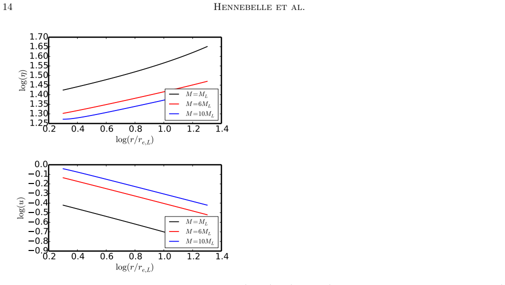
The load-bearing object is the first hydrostatic (Larson) core, with mass $M_L$ set by the dust opacity limit; the mechanism is the statistical counting of shielding fragments in the accreting envelope. The model takes the envelope density as $\rho_{\rm env}(r)=A c_s^2/(2\pi G r^2)$ and describes turbulent fluctuations by a log-normal PDF whose width is set by the local Mach number. Each fluctuation is tested with a virial criterion that includes self-gravity, the tidal fields of the core and envelope, thermal and turbulent support, and external thermal and ram-pressure surface terms fitted to the simulations. Counting fluctuations of mass at least $M_L$ in concentric shells gives the mean number of fragments $N(r)$; the radius where this number reaches a few defines the shielded accretion radius, and the distribution of unshielded mass peaks near $10M_L$.
What would settle it
Measure the thermal and ram pressure at the boundary of density fluctuations before they collapse, not on developed cores; if the resulting virial surface terms differ from the fits in Eq. (4) enough to move the radius where the mean fragment count reaches one away from $r\simeq 8\text{--}9\,r_{e,L}$, the predicted $10M_L$ peak shifts and the claimed agreement with the simulations fails.
Extended reading notes
Core claim
The central claim is that the peak of the stellar mass function is not inherited from the large-scale gas reservoir but generated during the final accretion phase. When the effective equation of state stiffens once dust becomes opaque, a first hydrostatic core of mass $M_L$ forms; because its cooling time is long, infalling gas piles up and the core grows. In the surrounding $r^{-2}$ envelope, turbulent density fluctuations that are at least as massive as $M_L$ and dense enough to overcome the tidal shear of the central core plus thermal, turbulent and ram-pressure support collapse into new fragments. These fragments accrete the gas beyond their own radii, so the final mass of the central object is set by the unshielded mass inside the radius where a few fragments have formed. Counting fluctuations analytically with a log-normal density PDF and a virial threshold gives a peak near $10M_L$; the two simulations show peaks at $0.1\text{--}0.2\,M_\odot$, i.e. $5\text{--}10M_L$, and suppressing sink formation within a few hundred AU shifts the distribution to twice larger masses.
Load-bearing premise
The calculation assumes that the pressure squeezing measured on already formed cores also acts on the less dense clumps that are about to become fragments; if the two situations differ, the predicted number of sibling fragments and the peak stellar mass would move.
Editorial extensions
If this is right
- The peak stellar mass should sit near $10M_L$, about $0.2\text{--}0.3\,M_\odot$ for solar-metallicity conditions, rather than being tied to the parent cloud's Jeans mass.
- The peak position should vary little across star-forming environments, because only the local envelope physics within a few hundred AU enters the calculation.
- Changing the effective equation of state so that $M_L$ changes should move the peak proportionally, as the simulations in this paper and its companions show.
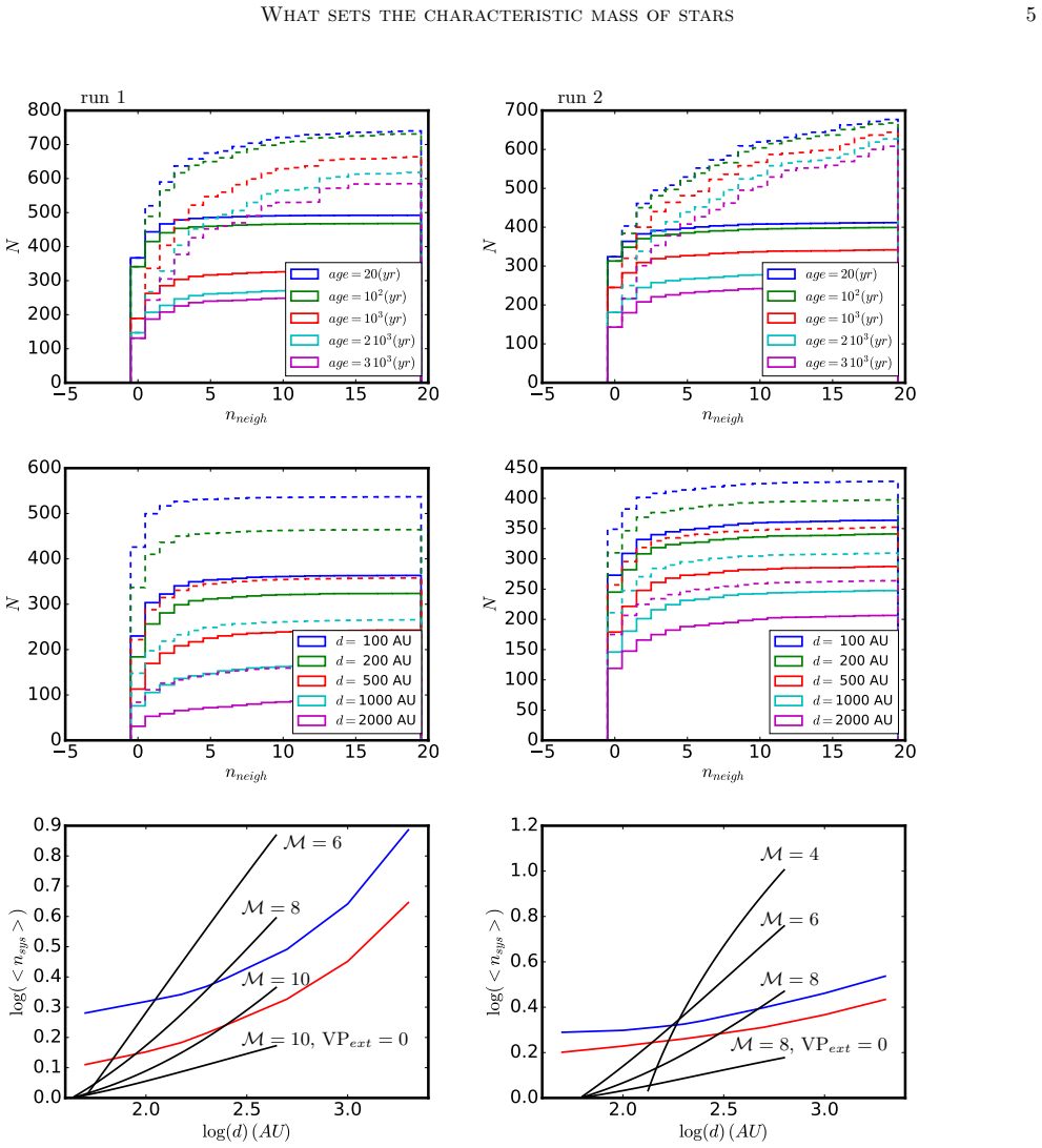
- Preventing fragmentation within a few hundred AU of existing protostars should shift the mass spectrum to about twice larger masses, matching the run1a and run1b experiments.
- The high-mass tail of the distribution is not explained by this shielding mechanism and is left to the initial mass-reservoir statistics.
Reading between the lines
- If the peak tracks $M_L$, resolved stellar mass functions in low-metallicity dwarf galaxies should show only a mild shift, because the paper's opacity scaling of $M_L$ is weak; this is a testable prediction beyond the paper's own metallicity discussion.
- Substellar objects may be the by-product of the same process: fragments below $M_L$ that cannot trigger the second collapse cool only if they stay isolated, otherwise they grow or merge into a first core.
- The same local shielding argument could apply at the high-mass end, where fragmentation-induced starvation has been invoked to limit accretion onto massive protostars, making the two regimes different scales of one competition.
- A direct numerical check of the model's key extrapolation would be to compute the virial surface terms on pre-collapse density fluctuations rather than on already formed cores; if those terms differ, the predicted fragment count and peak would need revision.
Signed reviews
Editorial analysis
A structured set of objections, weighed in public.
Referee Report
Summary. The paper proposes that the characteristic (peak) mass of the stellar IMF is set locally by the competition between accretion onto a first hydrostatic core (FHSC) and fragmentation of its surrounding collapsing envelope. Two AMR simulations of 1000 M_sun clumps with different initial conditions produce sink mass spectra peaking at about 0.1–0.2 M_sun, i.e. 5–10 times the FHSC mass M_L. Suppressing sink formation within 140 or 280 AU of existing sinks (run1a/run1b) shifts the peak upward by about a factor of two, supporting the fragmentation-starvation mechanism. An analytical model counts turbulent density fluctuations in the envelope that are self-gravitating against tidal, thermal, and pressure terms; the resulting unshielded-mass distribution peaks near 10 M_L, in apparent agreement with the simulations.
Significance. If the result holds, the paper provides a concrete, falsifiable mechanism for the universality of the IMF peak: the peak is tied to the FHSC mass and local envelope physics rather than to the large-scale Jeans mass. The run1a/run1b numerical experiments are a clean controlled test and are the strongest evidence in the paper. The analytical model is transparent and yields a testable relation between the peak mass and M_L, although it is not parameter-free. The authors also explicitly state several assumptions and limitations, including the extrapolation of surface-pressure fits from developed cores to core progenitors. The comparison to run2 with different initial conditions adds credibility, but the model's inputs remain partly calibrated on run1.
major comments (4)
- [§2.7, Eq. (4); §3.3.1] The fits in Eq. (4), VPext ≃ Eth(0.6−0.1M) and VPram ≃ Ekin(1.3−0.18M), become negative for M>6 and M>7.2, respectively. Yet §3.3.1 adopts M=8 for run1, so the virial threshold in Eq. (9) is evaluated with negative surface-pressure terms. Since negative VPext and VPram change the sign of the surface contribution, they artificially alter the critical density contrast ηcrit and therefore the fragment count N(r) that controls the predicted peak at about 10 M_L. The authors should state the Mach-number range over which the fits are valid, avoid extrapolating beyond it, or justify the negative values physically.
- [§2.7, §3.3] The surface-term fits used in Eq. (9) are derived from HOP cores identified at a density threshold of 10^8 cm^-3 (Fig. 6), i.e. from cores that are already formed and developed, but in §3.3 they are applied to pre-collapse density fluctuations that the authors themselves call "more core progenitors" (§3.3). This extrapolation is load-bearing: §3.3.2 reports that setting VPext=VPram=0 gives too few fragments, so the radius where the mean number of fragments N(r)=1, and hence the 10 M_L peak, depends on surface terms whose value for progenitors is not measured. A direct measurement of VPext and VPram for progenitor-type fluctuations, or a sensitivity study over their plausible range, is required to support the central prediction.
- [§3.3.2, Table 1] The model is calibrated on run1 (A=10, M=8, b=0.6) and then compared with the run1 peak, so the agreement between the predicted 10 M_L peak and the run1 spectrum is partly a consistency check rather than an independent prediction. The run2 comparison is a useful partial out-of-sample test, but it shares the same functional forms and several parameters. The authors should quantify the sensitivity of the predicted peak to A, b, ε, and nf over the ranges in Table 1, and ideally present the model prediction for an additional simulation before measuring the inputs.
- [Abstract; §4] The claim that the mass spectrum is "expected to be relatively universal" because the relevant processes are local is not established by the model itself: the inputs A, b, ε, and the VP fits are environmental parameters, and the paper only demonstrates insensitivity to two particular initial-condition choices. Unless the authors provide a physical argument or additional evidence that these parameters occupy a universal range, the universality conclusion should be softened to a speculation.
minor comments (4)
- [§2.2, §2.7] There are several typographical errors: "respectivelly" should be "respectively", the affiliation line contains "Universrté", and the Fig. 6 caption says "radio" where "ratio" is meant.
- [Fig. 3 caption] The caption should specify which black curve corresponds to which Mach number and to the VPext=0 case; currently the labels "M = 10, VPext = 0" and "M = 10" are ambiguous when read with multiple curves.
- [§3.2.5, Eq. (16)] The sentence preceding Eq. (16) is confusing: it first mentions mass located at radius smaller than the fragment position, then states that fragments accrete mass outside the sphere. Clarify that Eq. (16) follows from each fragment accreting a fraction 1/nf of the mass outside its radius.
- [§2.4] The description of the neighbour statistics says the maximum number of neighbours over timesteps is taken; please explain why the maximum rather than the mean or instantaneous value is used, as this choice could bias the inferred multiplicity.
Circularity Check
Peak at ~10 M_L is partly calibrated by run1-fitted surface-pressure terms, but remains an emergent count with independent run2 and sink-exclusion tests.
-
fitted input called prediction
[Section 2.7, Eq. (4); Section 3.2.3, Eq. (9); Section 3.3; Section 3.3.2]
"For the external pressure, we adopt a fit taken from section 2.7. Let us stress that those are typical values but that as seen from Fig. 5, large deviations from these values have been inferred, implying that in reality one should sum over a large number of configurations. Another limit is that Eqs. (4) are obtained for cores that are already formed and developed while the fluctuations we are identifying are more core progenitors."
Eqs. (4) fit VPext and VPram to run1 HOP cores (Fig. 6), and Section 3.2.3 puts them into the virial threshold Eq. (9): 'in the range ML <M < 10ML, we have the expressions stated by Eqs. (4).' The fragment count Eqs. (12)-(14) is then evaluated with run1-measured A=10, M=8, b=0.6, and the predicted peak is where N(r)=1 at r~9re,L, i.e. ~10ML. Section 3.3.2 states 'The model with VPext = VPram = 0 leads to too few fragments,' so the fitted surface terms are load-bearing. Thus the run1 peak at ~10ML is partly calibrated on run1 cores in the same mass range it predicts; the paper itself flags this as an extrapolation from developed cores to progenitor fluctuations.
full rationale
The main result is not a pure first-principles prediction: the external-pressure fits of Eqs. (4) are measured from run1 cores and are required to make the fragment count N(r) reach unity at the radius that yields the ~10 M_L peak; Section 3.3.2 says that with VP_ext=VP_ram=0 the model gives too few fragments. The paper itself (§3.3) flags the extrapolation from developed cores to progenitor fluctuations. This is a genuine partial circularity of the fitted-input kind, because the same run supplies both the fit and the peak used as the agreement test. I do not see the stronger forms of circularity: the peak at ~10 M_L is not equal by definition to any single input parameter; the analytical counting produces the peak from the probability distribution rather than returning a fitted number; run2 uses different initial conditions (A=7, Mach 4-8) and still gives reasonable agreement; and run1a/run1b are numerical experiments that test the shielding-fragmentation mechanism without using the analytical model. Citations to papers I and II are self-citations and supply the numerical peak and the gravitational-field expressions, but the present paper adds new simulations and quantitative comparisons, so they are not the sole load-bearing evidence. Score 4 reflects one load-bearing fitted input while the central claim retains independent content.
Assumptions & free parameters
free parameters (7)
- A (envelope density amplitude) =
5-10 (run1: 10, run2: 7)
- epsilon (turbulent energy fraction) =
0.3-1
- b (lognormal PDF width parameter) =
0.6-0.8
- n_f (number of shielding fragments) =
2-5
- alpha_turb (turbulent support coefficient) =
order of a few (Table 1: 0-1)
- Surface-term fits VP_ext and VP_ram =
VP_ext/E_th = 0.6 - 0.1 M; VP_ram/E_kin = 1.3 - 0.18 M
- H (virial factor for FHSC) =
0.5
assumptions (7)
- domain assumption The protostellar envelope density follows the collapsing-sphere profile rho proportional to r^-2 (Shu 1977), with amplitude A (Eq. 5).
- domain assumption Density fluctuations in the envelope are lognormally distributed with width sigma^2 = ln(1+b^2 M^2), and M is given by energy equipartition with gravity (Eqs. 7 and 8).
- domain assumption A density perturbation is unstable only if it satisfies the virial theorem including self-gravity, tidal forces from the central core and envelope, thermal and turbulent support, and external surface pressure (Eq. 9).
- domain assumption The minimum mass for fragmentation that leads to star formation is the first hydrostatic core mass M_L, about 0.02 to 0.03 M_sun, because smaller objects cool slowly and cannot trigger second collapse.
- ad hoc to paper A shielding fragment located at radius r_l accretes a fraction 1/n_f of the envelope mass outside its radius (Eq. 16).
- domain assumption The velocity dispersion inside a fluctuation scales as delta v proportional to delta r^0.5 (Eq. 11).
- domain assumption The envelope gas is approximately isothermal at the radii of interest (60-200 AU) even though the effective EOS stiffens at high densities.
Cite this review
Pith. "Pith review of How first hydrostatic cores, tidal forces and gravo-turbulent fluctuations set the characteristic mass of stars." pith.science (2026). https://pith.science/paper/JZRDTI5A
@misc{pith2026190807250,
  author       = {Pith},
  title        = {Pith review of: How first hydrostatic cores, tidal forces and gravo-turbulent fluctuations set the characteristic mass of stars},
  year         = {2026},
  howpublished = {\url{https://pith.science/paper/JZRDTI5A}},
  note         = {Machine review of arXiv:1908.07250}
}
read the original abstract
The stellar initial mass function (IMF) is playing a critical role in the history of our universe. We propose a theory that is based solely on local processes, namely the dust opacity limit, the tidal forces and the properties of the collapsing gas envelope. The idea is that the final mass of the central object is determined by the location of the nearest fragments, which accrete the gas located further away, preventing it to fall onto the central object. To estimate the relevant statistics in the neighbourhood of an accreting protostar, we perform high resolution numerical simulations. We also use these simulations to further test the idea that fragmentation in the vicinity of an existing protostar is determinant in setting the peak of the stellar mass spectrum. We develop an analytical model, which is based on a statistical counting of the turbulent density fluctuations, generated during the collapse, that are at least equal to the mass of the first hydrostatic core, and sufficiently important to supersede tidal and pressure forces to be self-gravitating. The analytical mass function presents a peak located at roughly 10 times the mass of the first hydrostatic core in good agreement with the numerical simulations. Since the physical processes involved are all local, i.e. occurs at scales of a few 100 AU or below, and do not depend on the gas distribution at large scale and global properties such as the mean Jeans mass, the mass spectrum is expected to be relatively universal.
Figures


Figures from the paper (6 more)




Reference graph
Works this paper leans on
-
[1]
, " * write output.state after.block = add.period write newline
ENTRY address archivePrefix author booktitle chapter doi edition editor eprint howpublished institution journal key month number organization pages publisher school series title misctitle type volume year version url label extra.label sort.label short.list INTEGERS output.state before.all mid.sentence after.sentence after.block FUNCTION init.state.consts ...
-
[2]
write newline
" write newline "" before.all 'output.state := FUNCTION format.url url empty "" new.block "" url * "" * if FUNCTION format.eprint eprint empty "" archivePrefix empty "" archivePrefix "arXiv" = new.block " " eprint * " " * new.block " " eprint * " " * if if if FUNCTION format.doi doi empty "" " " doi * " " * if FUNCTION format.pid doi empty eprint empty ""...
-
[4]
W., P \'e rez-Goytia , N., & Kuznetsova , A
Ballesteros-Paredes , J., Hartmann , L. W., P \'e rez-Goytia , N., & Kuznetsova , A. 2015, , 452, 566, 10.1093/mnras/stv1285
-
[5]
Bastian , N., Covey , K. R., & Meyer , M. R. 2010, , 48, 339, 10.1146/annurev-astro-082708-101642
-
[6]
2015, , 449, 2413, 10.1093/mnras/stv445
Basu , S., Gil , M., & Auddy , S. 2015, , 449, 2413, 10.1093/mnras/stv445
-
[7]
Basu , S., & Jones , C. E. 2004, , 347, L47, 10.1111/j.1365-2966.2004.07405.x
arXiv 2004
-
[8]
Bate , M. R. 1998, , 508, L95, 10.1086/311719
doi:10.1086/311719 1998
-
[9]
2009, , 392, 1363, 10.1111/j.1365-2966.2008.14165.x
---. 2009, , 392, 1363, 10.1111/j.1365-2966.2008.14165.x
arXiv 2009
Show all 56 references
- [10]
-
[11]
2014, , 445, 4015, 10.1093/mnras/stu2005
Bleuler , A., & Teyssier , R. 2014, , 445, 4015, 10.1093/mnras/stu2005
2014 doi
-
[12]
A., & Bate , M
Bonnell , I. A., & Bate , M. R. 2006, , 370, 488, 10.1111/j.1365-2966.2006.10495.x
2006
-
[14]
A., Smith , R
Bonnell , I. A., Smith , R. J., Clark , P. C., & Bate , M. R. 2011, , 410, 2339, 10.1111/j.1365-2966.2010.17603.x
2011
- [15]
-
[16]
J., Caselli , P., et al
di Francesco , J., Evans , II, N. J., Caselli , P., et al. 2007, Protostars and Planets V, 17
2007
-
[17]
2007, , 661, 262, 10.1086/513708
Dib , S., Kim , J., V \'a zquez-Semadeni , E., Burkert , A., & Shadmehri , M. 2007, , 661, 262, 10.1086/513708
2007 doi
- [18]
-
[19]
S., & Schmidt , W
Federrath , C., Klessen , R. S., & Schmidt , W. 2008, , 688, L79, 10.1086/595280
2008 doi
- [20]
-
[21]
2006, , 457, 371, 10.1051/0004-6361:20065371
Fromang , S., Hennebelle , P., & Teyssier , R. 2006, , 457, 371, 10.1051/0004-6361:20065371
2006 doi
-
[22]
Girichidis , P., Federrath , C., Banerjee , R., & Klessen , R. S. 2011, , 413, 2741, 10.1111/j.1365-2966.2011.18348.x
2011
-
[23]
R., & Hopkins , P
Guszejnov , D., Krumholz , M. R., & Hopkins , P. F. 2016, , 458, 673, 10.1093/mnras/stw315
2016 doi
-
[24]
2018, , 611, A24, 10.1051/0004-6361/201731071
Hennebelle , P. 2018, , 611, A24, 10.1051/0004-6361/201731071
2018 doi
-
[25]
2008, , 684, 395, 10.1086/589916
Hennebelle , P., & Chabrier , G. 2008, , 684, 395, 10.1086/589916
2008 doi
-
[26]
2012, , 20, 55, 10.1007/s00159-012-0055-y
Hennebelle , P., & Falgarone , E. 2012, , 20, 55, 10.1007/s00159-012-0055-y
2012 doi
-
[27]
P., Gladwin , P
Hennebelle , P., Whitworth , A. P., Gladwin , P. P., & Andr \'e , P. 2003, , 340, 870, 10.1046/j.1365-8711.2003.05584.x
2003
-
[28]
Hopkins , P. F. 2012, , 423, 2037, 10.1111/j.1365-2966.2012.20731.x
2012
- [29]
-
[30]
S., Larson , R
Jappsen , A.-K., Klessen , R. S., Larson , R. B., Li , Y., & Mac Low , M.-M. 2005, , 435, 611, 10.1051/0004-6361:20042178
2005 doi
-
[31]
2001, , 322, 231, 10.1046/j.1365-8711.2001.04022.x
Kroupa , P. 2001, , 322, 231, 10.1046/j.1365-8711.2001.04022.x
2001
-
[32]
R., Myers , A
Krumholz , M. R., Myers , A. T., Klein , R. I., & McKee , C. F. 2016, , 460, 3272, 10.1093/mnras/stw1236
2016 doi
-
[33]
Larson , R. B. 1969, , 145, 271
1969
-
[34]
2016, , 591, A30, 10.1051/0004-6361/201527981
Lee , Y.-N., & Hennebelle , P. 2016, , 591, A30, 10.1051/0004-6361/201527981
2016 doi
-
[35]
2018 a , , 611, A88, 10.1051/0004-6361/201731522
---. 2018 a , , 611, A88, 10.1051/0004-6361/201731522
2018 doi
-
[36]
2018 b , , 611, A89, 10.1051/0004-6361/201731523
---. 2018 b , , 611, A89, 10.1051/0004-6361/201731523
2018 doi
-
[37]
2019, , 622, A125, 10.1051/0004-6361/201834428
---. 2019, , 622, A125, 10.1051/0004-6361/201834428
2019 doi
-
[38]
1976, , 176, 367, 10.1093/mnras/176.2.367
Low , C., & Lynden-Bell , D. 1976, , 176, 367, 10.1093/mnras/176.2.367
1976 doi
-
[39]
N., Tomisaka , K., Matsumoto , T., & Inutsuka , S.-i
Machida , M. N., Tomisaka , K., Matsumoto , T., & Inutsuka , S.-i. 2008, , 677, 327, 10.1086/529133
2008 doi
-
[40]
A., Clarke , C
Maschberger , T., Bonnell , I. A., Clarke , C. J., & Moraux , E. 2014, , 439, 234, 10.1093/mnras/stt2403
2014 doi
-
[41]
1999, , 510, 822, 10.1086/306608
Masunaga , H., & Inutsuka , S.-i. 1999, , 510, 822, 10.1086/306608
1999 doi
-
[42]
M., & Inutsuka , S.-i
Masunaga , H., Miyama , S. M., & Inutsuka , S.-i. 1998, , 495, 346, 10.1086/305281
1998 doi
-
[43]
2015, , 804, 44, 10.1088/0004-637X/804/1/44
Murray , N., & Chang , P. 2015, , 804, 44, 10.1088/0004-637X/804/1/44
2015 doi
- [44]
-
[45]
Offner , S. S. R., Clark , P. C., Hennebelle , P., et al. 2014, Protostars and Planets VI, 53, 10.2458/azu_uapress_9780816531240-ch003
2014 doi
-
[46]
Padoan , P., Nordlund , A., & Jones , B. J. T. 1997, , 288, 145, 10.1093/mnras/288.1.145
1997 doi
-
[47]
S., & Mac Low , M.-M
Peters , T., Banerjee , R., Klessen , R. S., & Mac Low , M.-M. 2011, , 729, 72, 10.1088/0004-637X/729/1/72
2011 doi
-
[48]
Rees , M. J. 1976, , 176, 483, 10.1093/mnras/176.3.483
1976 doi
-
[49]
Salpeter , E. E. 1955, , 121, 161, 10.1086/145971
1955 doi
-
[50]
Saumon , D., Chabrier , G., & van Horn , H. M. 1995, , 99, 713, 10.1086/192204
1995 doi
-
[51]
2003, , 410, 611, 10.1051/0004-6361:20031279
Semenov , D., Henning , T., Helling , C., Ilgner , M., & Sedlmayr , E. 2003, , 410, 611, 10.1051/0004-6361:20031279
2003 doi
-
[52]
Shu , F. H. 1977, , 214, 488, 10.1086/155274
1977 doi
- [53]
-
[54]
2002, , 385, 337, 10.1051/0004-6361:20011817
Teyssier , R. 2002, , 385, 337, 10.1051/0004-6361:20011817
2002 doi
-
[55]
2018, , 477, 2220, 10.1093/mnras/sty798
Traficante , A., Duarte-Cabral , A., Elia , D., et al. 2018, , 477, 2220, 10.1093/mnras/sty798
2018 doi
-
[56]
2013, , 557, A90, 10.1051/0004-6361/201321423
Vaytet , N., Chabrier , G., Audit , E., et al. 2013, , 557, A90, 10.1051/0004-6361/201321423
2013 doi
-
[57]
2017, , 598, A116, 10.1051/0004-6361/201628194
Vaytet , N., & Haugb lle , T. 2017, , 598, A116, 10.1051/0004-6361/201628194
2017 doi
-
[58]
2007, Protostars and Planets V, 33
Ward-Thompson , D., Andr \'e , P., Crutcher , R., et al. 2007, Protostars and Planets V, 33
2007
Reviewed August 14, 2026 · model on record in the stance chip above.
Discussion (0). Continue with ORCID to comment.