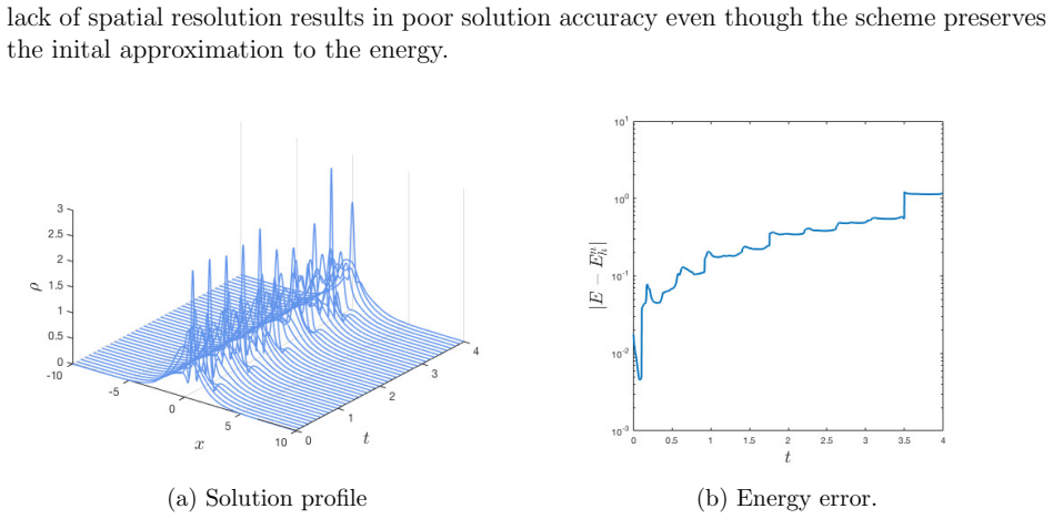
An hr-Adaptive Method for the Cubic Nonlinear Schr\"{o}dinger Equation
Pith reviewed 2026-05-25 08:51 UTC · model grok-4.3
The pith
An hr-adaptive method for the cubic nonlinear Schrödinger equation achieves second-order spatial convergence and user-controlled error tolerance.
A machine-rendered reading of the paper's core claim, the machinery that carries it, and where it could break.
Core claim
The hr-adaptive method, driven by a novel monitor function, solves the cubic NLSE in one space dimension such that the spatial error remains below a user-specified tolerance and the observed convergence rate is second order, outperforming other moving-mesh approaches in solution accuracy.
What carries the argument
The hr-adaptive procedure that couples r-adaptive node movement with h-adaptive local refinement, using a novel monitor function to generate the adaptive mesh.
If this is right
- Spatial error stays within the tolerance supplied by the user.
- Second-order spatial convergence is obtained for the cubic NLSE.
- Solution accuracy exceeds that of pure moving-mesh schemes on comparable node counts.
- The method adapts automatically when solution features become steeper or smoother over time.
Where Pith is reading between the lines
- The same monitor-function construction may extend to other dispersive or nonlinear wave equations that develop localized steep gradients.
- Error control via the tolerance parameter could reduce computational cost for long-time integrations compared with uniform meshes.
- The hr-strategy offers a route to three-dimensional extensions where pure r-adaptation alone becomes insufficient.
Load-bearing premise
The novel monitor function produces a mesh that simultaneously delivers the claimed error control and the observed second-order spatial convergence for the cubic NLSE.
What would settle it
A numerical test in which the computed spatial error exceeds the user tolerance or the observed convergence rate drops below second order when the novel monitor function is employed.
Figures
read the original abstract
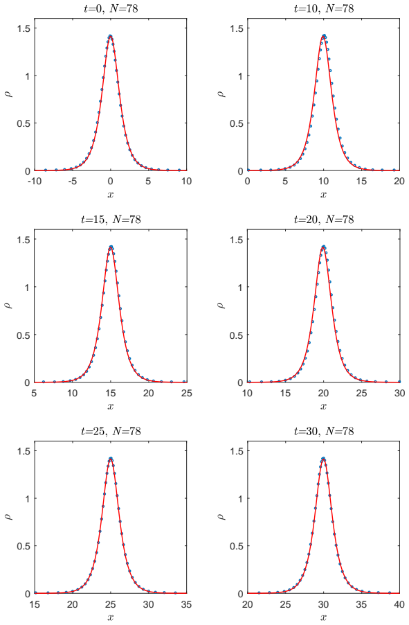
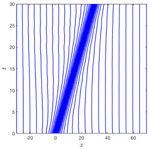
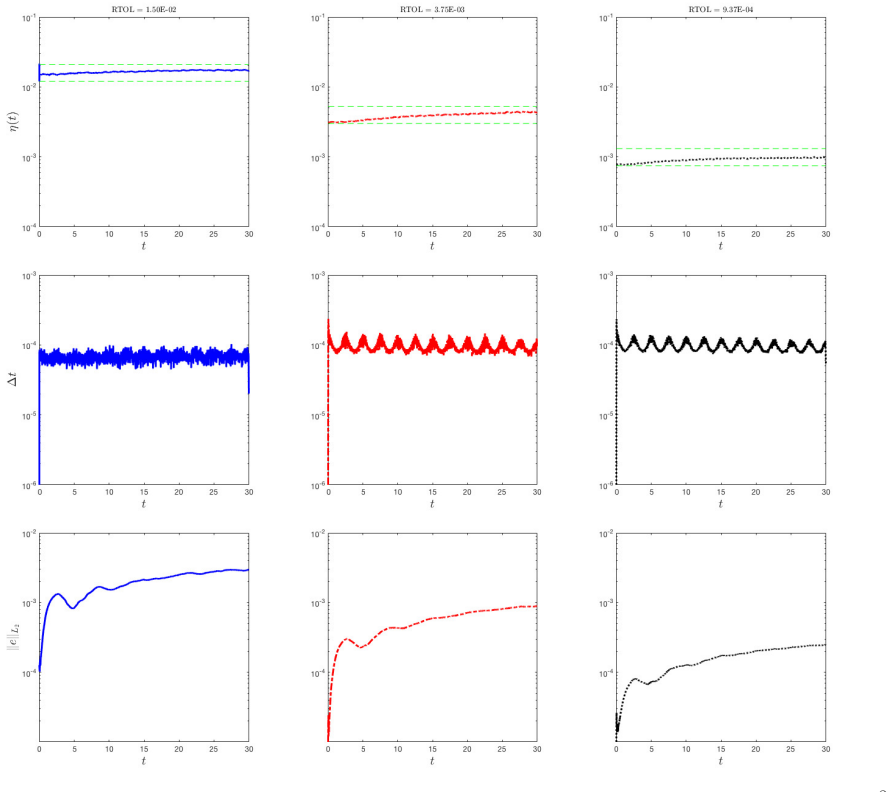
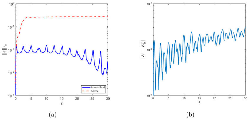
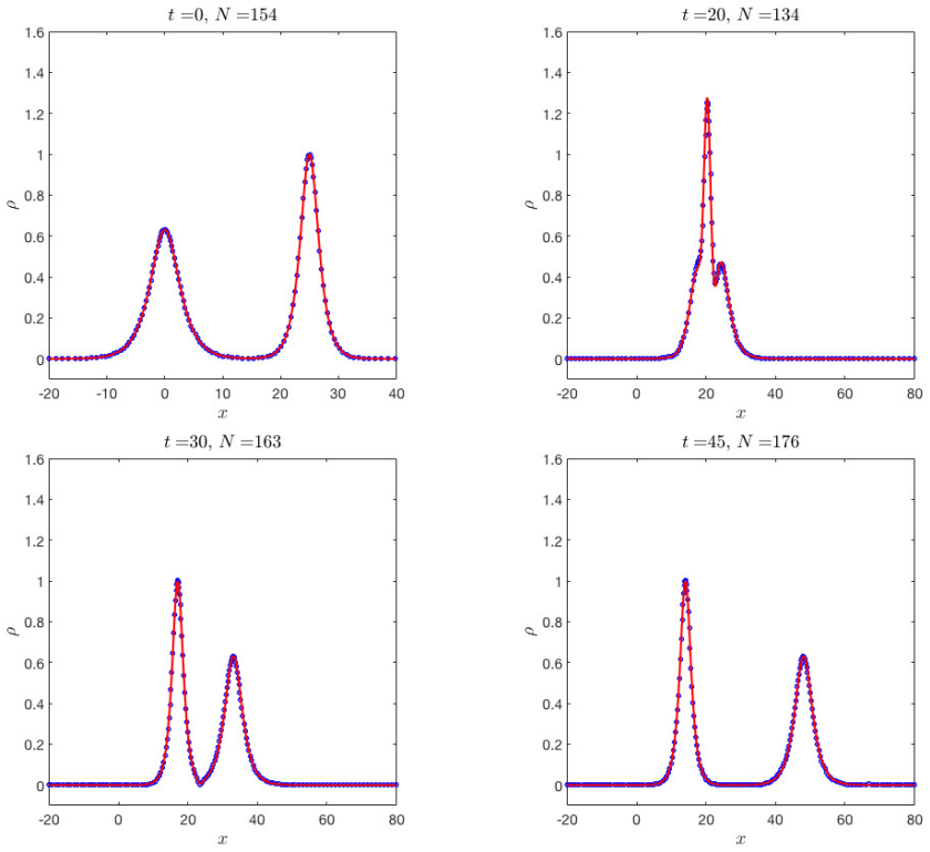
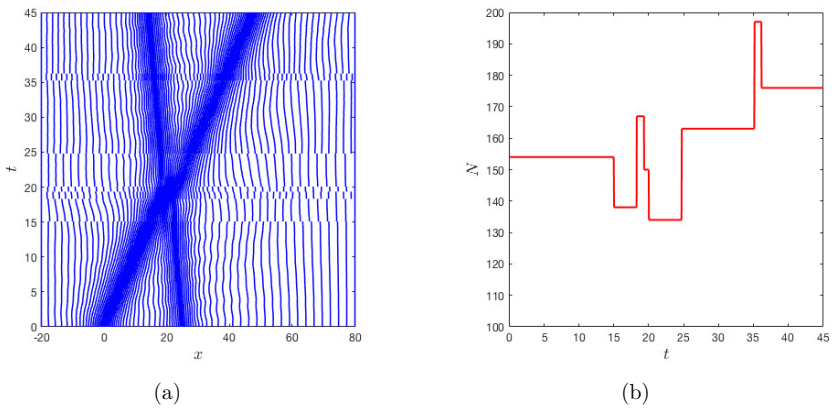
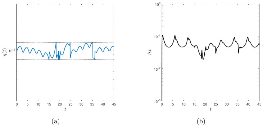
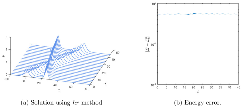
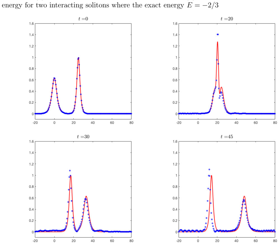
The nonlinear Schr\"{o}dinger equation (NLSE) is one of the most important equations in quantum mechanics, and appears in a wide range of applications including optical fibre communications, plasma physics and biomolecule dynamics. It is a notoriously difficult problem to solve numerically as solutions have very steep temporal and spatial gradients. Adaptive moving mesh methods ($r$-adaptive) attempt to optimise the accuracy obtained using a fixed number of nodes by moving them to regions of steep solution features. This approach on its own is however limited if the solution becomes more or less difficult to resolve over the period of interest. Mesh refinement methods ($h$-adaptive), where the mesh is locally coarsened or refined, is an alternative adaptive strategy which is popular for time-independent problems. In this paper, we consider the effectiveness of a combined method ($hr$-adaptive) to solve the NLSE in one space dimension. Simulations are presented indicating excellent solution accuracy compared to other moving mesh approaches. The method is also shown to control the spatial error based on the user's input error tolerance. Evidence is also presented indicating second-order spatial convergence using a novel monitor function to generate the adaptive moving mesh.
Editorial analysis
A structured set of objections, weighed in public.
Referee Report
Summary. The paper presents an hr-adaptive finite-difference method for the one-dimensional cubic nonlinear Schrödinger equation that combines r-adaptation (moving mesh generated by a novel monitor function) with h-adaptation (local refinement/coarsening). Simulations are reported to demonstrate that the method controls the spatial error to a user-specified tolerance, achieves second-order spatial convergence, and yields higher accuracy than other moving-mesh approaches.
Significance. If the monitor-function construction and associated error estimates are shown to be sound, the work supplies a practical adaptive strategy for dispersive problems whose solutions develop localized steep gradients. The explicit demonstration of user-controlled spatial error is a useful practical contribution for applications in optics and quantum mechanics.
major comments (3)
- [§3.2] §3.2 (monitor-function construction): the novel monitor function is introduced without an explicit equidistribution principle or truncation-error analysis showing that the quantity being equidistributed yields a local truncation error of O(h²) for the underlying spatial discretization of the cubic NLSE; this is load-bearing for both the claimed second-order convergence and the error-control property.
- [§4.3] §4.3 (convergence experiments): the reported second-order rates and error-tolerance results rest on simulations whose reference solutions, error norms, and mesh-velocity coupling are not described in sufficient detail to confirm that order reduction does not occur at h-refinement interfaces or from the r-adaptation velocity term.
- [§3.3] §3.3 (hr-coupling): no analysis or numerical test is supplied to verify that the combined h- and r-adaptation preserves the formal order when the monitor function is recomputed after each h-refinement step.
minor comments (2)
- [Figure 5] Figure 5 caption should state the precise norm and reference solution used for the plotted errors.
- [§2] A short paragraph comparing the novel monitor to the standard arc-length or curvature monitors used in prior moving-mesh NLSE papers would improve context.
Simulated Author's Rebuttal
We thank the referee for the careful reading and constructive comments. We address each major point below and will revise the manuscript to incorporate the requested clarifications and supporting material.
read point-by-point responses
-
Referee: [§3.2] §3.2 (monitor-function construction): the novel monitor function is introduced without an explicit equidistribution principle or truncation-error analysis showing that the quantity being equidistributed yields a local truncation error of O(h²) for the underlying spatial discretization of the cubic NLSE; this is load-bearing for both the claimed second-order convergence and the error-control property.
Authors: We agree that an explicit derivation linking the monitor function to the equidistribution principle and a truncation-error analysis would strengthen the presentation. In the revised manuscript we will add a dedicated subsection deriving the monitor function from an equidistribution principle and providing a truncation-error analysis that confirms the local truncation error remains O(h²) for the underlying second-order spatial discretization of the cubic NLSE. revision: yes
-
Referee: [§4.3] §4.3 (convergence experiments): the reported second-order rates and error-tolerance results rest on simulations whose reference solutions, error norms, and mesh-velocity coupling are not described in sufficient detail to confirm that order reduction does not occur at h-refinement interfaces or from the r-adaptation velocity term.
Authors: We acknowledge that the current description of the numerical experiments is insufficient to allow independent verification of the reported orders. In the revision we will expand §4.3 with: (i) explicit statements of how reference solutions are generated (high-resolution fixed-mesh computations or exact solutions where available), (ii) the precise error norms used, and (iii) a description of the mesh-velocity term treatment and its handling at h-refinement interfaces, together with additional numerical checks confirming that order reduction does not occur. revision: yes
-
Referee: [§3.3] §3.3 (hr-coupling): no analysis or numerical test is supplied to verify that the combined h- and r-adaptation preserves the formal order when the monitor function is recomputed after each h-refinement step.
Authors: We agree that a direct verification of order preservation under the combined hr-adaptation is desirable. The revised manuscript will include a new numerical test that recomputes the monitor function after each h-refinement step and reports the observed convergence rates, thereby confirming that the formal second-order accuracy is retained. revision: yes
Circularity Check
No significant circularity detected
full rationale
The paper presents an hr-adaptive numerical method for the cubic NLSE as an independent algorithmic construction, with claims of error control and second-order convergence supported by simulations using a novel monitor function. No equations, parameter fits, or self-citations in the abstract or described claims reduce any reported result to a tautology by construction. The monitor function is introduced as part of the method rather than defined in terms of the target convergence order, and no load-bearing self-citation chains or ansatz smuggling are identifiable from the given text. This is the most common honest finding for a methods paper whose central claims rest on external simulation evidence rather than internal redefinition.
Axiom & Free-Parameter Ledger
Reference graph
Works this paper leans on
-
[1]
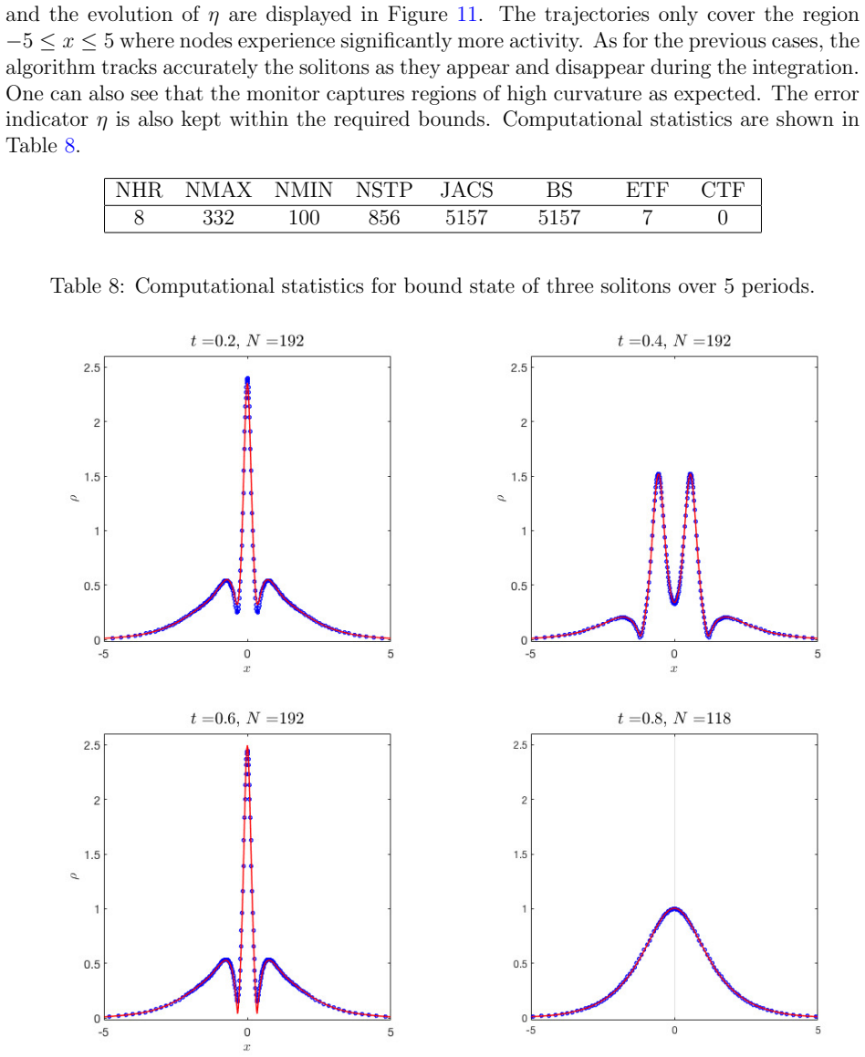
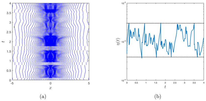
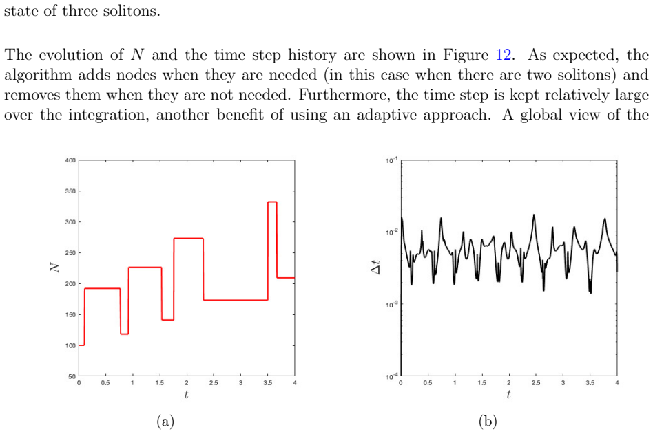
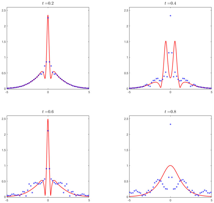
S. Adjerid and J. E. Flaherty. A moving finite element method with error estimation and refinement for one-dimensional time dependent partial differential equations. SIAM 24 Figure 14: Numerical solution (circles) and reference solution (line) for the bound state of three solitons using MCN scheme and a uniform mesh with N = 210. J. Numer. Anal. , 23(4):778–...
work page 1986
-
[2]
B. A. Ammons and M. Vable. An HR-method of mesh refinement for boundary element method. Int. J. Numer. Meth. Eng. , 43(6):979–996, 1998
work page 1998
-
[3]
L. Barletti, L. Brugnano, G. Frasca Caccia, and F. Iavernaro. Energy-conserving meth- ods for the nonlinear Schr¨ odinger equation.Appl. Math. Comput. , 318:3–18, 2018
work page 2018
-
[4]
G. Beckett and J. A. Mackenzie. Convergence analysis of finite difference approxima- tions on equidistributed grids to a singularly perturbed boundary value problem. Appl. Numer. Math., 35:87–109, 2000
work page 2000
-
[5]
G. Beckett, J. A. Mackenzie, A. Ramage, and D. M. Sloan. On the numerical solution of one-dimensional PDEs using adaptive methods based on equidistribution. J. Comput. Phys., 167:372–392, 2001. 25
work page 2001
-
[6]
G. Beckett, J. A. Mackenzie, and M. L. Robertson. A moving mesh finite element method for the solution of two-dimensional Stefan problems.J. Comput. Phys., 168:500– 518, 2001
work page 2001
-
[7]
C. J. Budd, S. Chen, and R. D. Russell. New self-similar solutions of the nonlinear Schr¨ odinger equation with moving mesh computations.J. Comput. Phys. , 152(2):756 – 789, 1999
work page 1999
-
[8]
C. J. Budd, W. Huang, and R. D. Russell. Adaptivity with moving grids.Acta Numerica, 18:111–241, 2009
work page 2009
-
[9]
W. Cao, W. Huang, and R. D. Russell. Comparison of two-dimensional r-adaptive finite element methods using various error indicators. Math. Comput. Simulat. , 56:127–143, 2001
work page 2001
-
[10]
W. Cao, W. Huang, and R. D. Russell. Approaches for generating moving adaptive meshes: location versus velocity. Appl. Numer. Math. , 47(2):121 – 138, 2003. Second International Workshop on Numerical Linear Algebra - Numerical Methods for Partial Differential Equations and Optimization
work page 2003
- [11]
-
[12]
Good approximation by splines with variable knots II
Carl de Boor. Good approximation by splines with variable knots II. In Springer Lecture Notes Series, 363. Springer-Verlag, 1973
work page 1973
-
[13]
M. Delfour, M. Fortin, and G. Payre. Finite-difference solutions of a non-linear Schr¨ odinger equation.J. Comput. Phys. , 44:277–288, 1981
work page 1981
-
[14]
Z. Fei, V. M. P´ erez-Garc´ ıa, and L. V´ azquez. Numerical simulation of nonlinear Schr¨ odinger systems: A new conservative scheme. Appl. Math. Comput. , 71:165–177, 1995
work page 1995
- [15]
-
[16]
E. Hairer and G. Wanner. Solving Ordinary Differential Equations II Stiff and Differential-Algebraic Problems. Springer, Berlin, 1991
work page 1991
-
[17]
D. F. Hawken, J. J. Gottlieb, and J. S. Hansen. Review of some adaptive node-movement techniques in finite-element and finite-difference solutions of partial differential equa- tions. J. Comput. Phys. , 95:254–302, 1991
work page 1991
-
[18]
B. M. Herbst, J. Ll. Morris, and A. R. Mitchell. Numerical experience with the nonlinear schr¨ odinger equation.J. Comput. Phys. , 60:282–305, 1985
work page 1985
-
[19]
F. Hu, R. Wang, X. Chen, and H. Feng. An adaptive mesh method for 1D hyperbolic conservation laws. Appl. Numer. Math. , 91:11–25, 2015
work page 2015
-
[20]
W. Huang. Practical aspects of formulation and solution of moving mesh partial differ- ential equations. J. Comput. Phys. , 171:753, 2001. 26
work page 2001
- [21]
- [22]
-
[23]
W. Huang and R. D. Russell. Moving mesh strategy based on a gradient flow equation for two-dimensional problems. SIAM J. Sci. Comput. , 20(3):998–1015, 1999
work page 1999
-
[24]
W. Huang and R. D. Russell. Adaptive mesh movement - the MMPDE approach and its applications. J. Comput. Appl. Math. , 128:383–398, 2001
work page 2001
-
[25]
E. Kita, K. Higuchi, and N. Kamiya. r- and hr-adaptive boundary element method for two-dimensional potential problem. Computers & Structures , 74(1):11–19, 2000
work page 2000
- [26]
-
[27]
R. Li, T. Tang, and P. Zhang. Moving mesh methods in multiple dimensions based on harmonic maps. J. Comput. Phys. , 170(2):562 – 588, 2001
work page 2001
-
[28]
J. A. Mackenzie and W. R. Mekwi. On the use of moving mesh methods to solve PDEs. In T. Tang and J. Xu, editors, Adaptive Computations: Theory and Algorithms , pages 242–278. Science Press, Beijing, 2007
work page 2007
-
[29]
John W Miles. An envelope soliton problem. SIAM J. Appl. Math. , 41(2):227–230, October 1981
work page 1981
-
[30]
W. F. Mitchell and M. A. McClain. A Survey of hp-Adaptive Strategies for Elliptic Partial Differential Equations , pages 227–258. Springer Netherlands, 2011
work page 2011
-
[31]
L. S. Mulholland, Y. Qiu, and D. M. Sloan. Solution of evolutionary partial differen- tial equations using adaptive finite differences with pseudospectral post-processing. J. Comput. Phys., 131:280–298, 1997
work page 1997
-
[32]
B. Ong, R. Russell, and S. Ruuth. An hr moving mesh method for one-dimensional time-dependent PDEs. In Proceedings of 21st International Meshing Roundtable, pages 39–54. Springer Berlin Heidelberg, 2013
work page 2013
-
[33]
M.D. Piggott, C.C. Pain, G.J. Gorman, P.W. Power, and A.J.H. Goddard. h, r, and hr adaptivity with applications in numerical ocean modelling. Ocean Modelling, 10(1):95 – 113, 2005
work page 2005
-
[34]
M. A. Revilla. Simple time and space adaptation in one-dimensional evolutionary partial differential equations. Int. J. Numer. Meth. Eng. , 23:2263–2275, 1986
work page 1986
-
[35]
J. M. Sanz-Serna. Methods for the numerical solution of the nonlinear Schroedinger equation. Math. Comput., 43(167):21–27, 1984
work page 1984
-
[36]
J. M. Sanz-Serna and I. Christie. A simple adaptive technique for nonlinear wave problems. J. Comput. Phys. , 67:348–360, 1986. 27
work page 1986
-
[37]
J. M. Sanz-Serna and V. S. Manoranjan. A method for the integration in time of certain partial differential equations. J. Comput. Phys. , 52:273–289, 1983
work page 1983
-
[38]
J. M. Sanz-Serna and J. G. Verwer. Conservative and nonconservative schemes for the solution of the nonlinear Schr¨ odinger equation.IMA J. Numer. Anal. , 6:25–42, 1986
work page 1986
- [39]
-
[40]
T. R. Taha and M. J. Ablowitz. Analytical and numerical aspects of certain nonlinear evolution equations. II. numerical, nonlinear Schr¨ odinger equation. J. Comput. Phys. , 55:203–230, 1984
work page 1984
-
[41]
Z. Tan, Z. Zhang, Y. Huang, and T. Tang. Moving mesh methods with locally varying time steps. J. Comput. Phys. , 200:347–367, 2004
work page 2004
-
[42]
H. Tang and T. Tang. Adaptive mesh methods for one- and two-dimensional hyperbolic conservation laws. SIAM J. Numer. Anal. , 41(2):487–515, 2003
work page 2003
-
[43]
T. Tang. Moving mesh methods for computational fluid dynamics. Contemporary Mathematics, 383:141–174, 2005
work page 2005
-
[44]
A. Vande Wouwer, Ph. Saucez, and W. E. Schiesser, editors. Adaptive Method of Lines. Chapman & Hall/CRC, 2001
work page 2001
-
[45]
J. G. Verwer, J. G. Blom, and J. M. Sanz-Serna. An adaptive moving grid method for one-dimensional systems of partial differential equations. J. Comput. Phys., 82:454–486, 1989
work page 1989
-
[46]
P. Wang and C. Huang. An energy conservative difference scheme for the nonlinear fractional Schr¨ odinger equations.J. Comput. Phys. , 293:238 – 251, 2015
work page 2015
-
[47]
G. B. Whitham. Linear and Nonlinear Waves . John Wiley & Sons, 1974
work page 1974
-
[48]
S. Xie, G. Li, and S. Yi. Compact finite difference schemes with high accuracy for one- dimensional nonlinear Schr¨ odinger equation. Comput. Methods Appl. Mech. Engrg. , 198(9-12):1052 – 1060, 2009
work page 2009
-
[49]
Z. Zhang and T. Tang. An adaptive mesh redistribution algorithm for convection- dominated problems. Commun. Pur. Appl. Ana. , 1(3):341–357, 2002. 28
work page 2002
discussion (0)
Sign in with ORCID, Apple, or X to comment. Anyone can read and Pith papers without signing in.