REVIEW 4 major objections 6 minor 23 references
Parameter optimization for restarted mixed precision iterative sparse solver
T0 review · 4 major / 6 minor · reviewed 2026-08-11 · deepseek-v4-flash
Pith's one-line read This paper proposes that the optimal single-precision stopping tolerance for a two-stage mixed-precision CG solve can be predicted from cheap matrix features, chiefly the sparsity graph diameter, cutting equivalent double-precision work…
desk verdict A well-run empirical study of kNN-based precision switching in mixed-precision CG, but the paper's central mechanistic claim about graph diameter controlling rounding error growth is contradicted by its own dense right-hand sides. read the letter →
The pith
A machine-rendered reading of the paper's core claim, the machinery that carries it, and where it could break.
The reading
What carries the argument
The mechanism that carries the argument is the error expansion $e_k = (I + \sum_{t=1}^k \gamma_t^{(k)} A^t) e_0$, which expresses the CG error at iteration $k$ as a polynomial in the system matrix acting on the initial error. Because the sparsity pattern of $A^t$ is contained in the sparsity pattern of the $t$-th power of the adjacency matrix, the graph diameter $\ell$ controls how many powers stay sparse: for $t<\ell$, $A^t$ is still sparse, so residuals and search directions tend to stay sparse and rounding errors accumulate slowly. The paper operationalizes this by estimating the diameter with the 2BFS pseudo-diameter $\tilde{\ell}$ (two breadth-first searches, $O(m)$ work) and combining $\tilde{\ell}$ with the matrix size $n$, the number of nonzeros $m$, and the early single-precision residual decay rate $v$ into a four-component feature vector $\chi(A)=(n,m,\tilde{\ell},v)$. A distance-weighted k-nearest-neighbors classifier assigns one of six candidate tolerances $\varepsilon_1\in\{10^{-2},\ldots,10^{-7}\}$; the whole parameter-estimation overhead is bounded by 1% of a full double-precision CG solve via clock-cycle estimates.
What would settle it
Construct two symmetric positive definite sparse matrices with the same condition number but very different sparsity-graph diameters, for example a path-like matrix and a star-like matrix with matched spectra via diagonal scaling, and measure the iteration at which single-precision CG residuals stagnate on dense right-hand sides: if the large-diameter matrix does not allow more single-precision iterations than the small-diameter one, the diameter-based switching rule is not doing the work claimed.
Extended reading notes
Core claim
On its own terms, the paper's central claim is that the sparsity graph diameter of a symmetric positive definite sparse matrix is a genuinely informative predictor of rounding-error growth in finite-precision CG, and that it can be used to set the single-precision stopping tolerance $\varepsilon_1$ in a two-stage mixed-precision solve. The argument runs through the error expansion $e_k = (I + \sum_{t=1}^k \gamma_t^{(k)} A^t) e_0$: because $A^t$ has nonzero entries only where the $t$-th power of the adjacency graph has walks, a large graph diameter delays fill-in and delays the densification of Krylov vectors, so rounding errors accumulate more slowly in early single-precision iterations. The paper reports that, across three matrix types, the resulting algorithm cuts equivalent double-precision iterations by roughly 22%, 22%, and 17.7% when the single-to-double iteration time ratio is fixed at 1:3, and by up to about 31% when that ratio is measured per matrix, always within 1.5% of the optimal-tolerance oracle. It also reports that the diameter effect persists for Jacobi iterations, whose transition matrix shares the system matrix's graph, but not for Gauss–Seidel, and that for well-conditioned banded matrices the diameter no longer controls efficiency.
Load-bearing premise
The load-bearing premise is that the sparsity pattern of powers of the matrix, captured by the sparsity graph diameter, controls how fast rounding errors accumulate in finite-precision CG, so that a large diameter genuinely allows more safe single-precision iterations; if Krylov vectors densify rapidly even when the diameter is large, the predicted link weakens.
Editorial extensions
If this is right
- If the claim holds, mixed-precision CG can choose its switching tolerance automatically from matrix structure, removing trial-and-error tuning.
- The near-oracle performance, within 1.5% of the optimal tolerance, means the cheap classifier does not sacrifice the speedup that a perfect choice of $\varepsilon_1$ would give.
- The diameter effect is expected to persist when a graph-preserving preconditioner such as Jacobi is used, extending the method to matrices with condition numbers above 1000.
- Because the Jacobi transition matrix shares the system matrix's graph, the same diameter-based staging applies to Jacobi iterations, while Gauss–Seidel and relaxation methods should not be expected to show the same dependence.
- The reported efficiency increases with matrix size, so the algorithm becomes more attractive for large sparse problems.
Reading between the lines
- Not stated in the paper: the same feature vector might predict stagnation points in lower-precision CG generally, not just the two-stage switch, since the graph-diameter effect is about rounding-error accumulation rather than about CG specifically.
- The paper's experiments use dense right-hand sides; a natural test is whether the diameter-based schedule still holds for sparse or structured right-hand sides, where Krylov vectors may stay sparse for different reasons.
- The 1% overhead bound relies on sequential clock-cycle estimates; on parallel or GPU hardware the relative cost of computing the pseudo-diameter and running kNN could change, though the paper notes parallel variants should not degrade the estimate.
- One could test the diameter hypothesis directly by comparing two matrices with identical spectra but different sparsity graph diameters, isolating diameter from condition number.
Signed reviews
Editorial analysis
A structured set of objections, weighed in public.
Referee Report
Summary. The paper considers a two-stage mixed-precision conjugate gradient (CG) solver for sparse symmetric positive definite systems: single-precision CG runs to a switching tolerance epsilon_1, then double-precision CG refines the solution to a final tolerance epsilon_2. The switching tolerance is selected by a k-nearest-neighbors classifier over a feature vector (n, m, pseudo-diameter of the matrix sparsity graph, and the average residual decay rate during the first k_0 single-precision iterations), with training labels obtained by exhaustive evaluation of six candidate epsilon_1 values on generated matrices. The paper claims an average reduction of more than 17% in equivalent double-precision CG iterations, a gap of at most 1.5% relative to the oracle choice of epsilon_1, overhead below 1% of the double-precision solve time, and a novel conceptual result: that the sparsity-graph diameter influences rounding-error growth in CG. Experiments cover three families of sparse matrices (extended stars with random edges, random sparse graphs, and banded matrices) with n up to 1000.
Significance. If the empirical results hold, the practical contribution is a cheap, near-oracle precision-switch rule backed by a consistent evaluation pipeline: optimal labels are computed on training matrices only, predictions are evaluated on held-out test matrices, standard deviations are reported, and the cost model deliberately uses a pessimistic omega = 1/3 iteration-time ratio. The complexity accounting for the pseudo-diameter (2BFS) and for kNN is explicit, and the efficiency evaluation is not circular. However, the advertised novelty—the graph-diameter mechanism and the diameter feature—is the least supported part of the paper: the proposed causal mechanism is contradicted by the paper's own dense right-hand sides, and no ablation quantifies the diameter's predictive contribution beyond the other features. The empirical scheme may remain viable, but the central conceptual claim and the abstract's quantitative claims require substantial correction.
major comments (4)
- [Section 5 (Eq. (13)); Sections 2 and 5.1] The central mechanism claim is contradicted by the paper's own experimental setup. Section 5 argues that for t < l the power A^t remains sparse and hence "Krylov vectors (e.g., residuals and search directions) tend to stay sparse as well", so that rounding errors accumulate more slowly for large-diameter graphs. But in the experiments the right-hand side is dense: in Section 2, b = Ax with x drawn uniformly from (1,2), and in the star/path illustrations of Section 5.1, b = A(1,...,1). Since x_0 = 0, the initial error e_0 = x_hat is dense, r_0 = A e_0 is dense, and every subsequent residual or search direction is dense after one sparse matrix-vector product. In Eq. (13), e_k = (I + sum_t gamma_t A^t) e_0, the vectors A^t e_0 are dense for t >= 1 regardless of the sparsity pattern of A^t; the diameter of the sparsity graph is therefore irrelevant to the density of the iterates in these experiments. The conclusion that delayed fill-in implies slower rounding-error accumulation does not follow. In addition, the star/path comparison (Figs. 2-3, Tables 4-5) is confounded: the modified star matrix has an eigenvalue of multiplicity n-2, so the CG minimal polynomial has degree three, which alone explains the small N_1 values (N_1 = 4 for the star), while the path matrix has distinct eigenvalues and a much larger condition number. The observed difference does not isolate the diameter. The abstract's "we show" claim about the diameter influencing rounding-error growth needs either a corrected argument or a control experiment (e.g., equal spectra with different graph diameters).
- [Section 5.1 (Tables 1-3); Section 8.1] The predictive contribution of the diameter feature is never isolated. The kNN feature vector includes the residual-decay rate v (Eq. (15)), which is a strong proxy for the eigenvalue distribution and hence for CG convergence and attainable accuracy; n and m are also included. No ablation is reported (e.g., classification with and without the pseudo-diameter, or with and without v), so the roughly 70% classification accuracy and the near-oracle efficiency could be driven entirely by v, with the diameter contributing nothing. The cross-tabulations in Tables 1-3 do not resolve this: within a condition-number band, efficiency and pseudo-diameter are correlated, but both are functions of the same construction parameters (mu, ray length and number of rays, number of added random edges), which also control the spectrum and its multiplicity structure. Moreover, Table 3's well-conditioned banded row shows the opposite association: the above-average-efficiency subset has M_l_tilde = 39.7 versus 66.5 for the below-average subset, a non-monotonicity the paper mentions but does not explain. An ablation study and a control for spectral confounders are needed before the novelty claim—that graph diameter is a useful predictive feature for precision switching—can be accepted.
- [Abstract; Section 10.3; Tables 21-22] The abstract's quantitative claim that the speedup is "at most 1.5% worse than that achieved with the optimal (oracle) choice of epsilon_1" is inconsistent with the reported data. Section 10.3 states that the gap does not exceed 3.0%, 1.5%, and 1.5% for the three matrix types, and Table 21 (extended stars, n = 1001, omega = 1/3) shows gaps of 3.09 to 4.15 percentage points (e.g., k = 5: 18.71 vs 22.86). Even for the augmented sample in Table 23 the gap reaches 2.64 points. Furthermore, Table 22 (k = 20) reports ME = 27.41 versus ME_opt = 27.20, which violates the definitional inequality E <= E_opt from Section 10.2 and indicates an error in that cell. The abstract, Section 10.3, and the tables must be reconciled before the headline claims can be considered accurate.
- [Section 6 (Eq. (15)), Remark 2; Eqs. (3)-(4)] The cost model used for the efficiency claims omits part of the cost of computing the feature v, and the experiments omit its parameter k_0. Remark 2 states that "the residual norms ||r_i||_2 for i <= k_0 are computed in double precision", which requires an extra double-precision matrix-vector product and norm per probing iteration; the same remark claims this "does not require any computations beyond those already performed by the algorithm", which is inconsistent with the stated double-precision residual computation. The efficiency metric in Eqs. (3)-(4) counts only single-precision iterations N_1 (weighted by omega) plus N_2, so the extra double-precision work in the first k_0 iterations is not reflected in the reported savings; depending on k_0, this could reduce the claimed 17-31% efficiencies by a non-negligible amount. In addition, k_0 is never specified: Section 6 only says it is "determined in advance by sampling", and no value appears in the experimental sections. The authors should report k_0, state how it was chosen, and account for the probing cost in Eqs. (3)-(4).
minor comments (6)
- [Section 8.1, 8.4, Table captions] There are several typos: "detremine" in Section 8.1, "is consists" in Section 8.4, and "effficiency" in the Table captions; a proofreading pass is needed.
- [Section 14 (end) vs. Algorithm II / Section 8.1] The appendix states that "a 3-dimensional feature vector (m, l_tilde, v) - excluding matrix size n - was used in the experiments", which contradicts Algorithm II and Section 8.1, where the feature vector is defined as chi(A) = (n, m, l_tilde, v). Clarify which feature vector was used in each experiment.
- [Section 9] Section 9 reports "extensive computational experiments" with a multilayer perceptron but provides no numerical results, no accuracy figures, and no direct comparison with kNN; either include the data or present the claim as a conjecture.
- [Tables 1-3 captions] The captions say the second column group contains ME and N for the below-average-efficiency subset, but the table columns contain M_l_tilde and N; align the caption text with the actual column layout.
- [Section 7.2] The cycle-counting model for comparing BFS cost with CG cost ignores memory traffic, which typically dominates the runtime of BFS on irregular sparse graphs; the "well below 1%" overhead claim should acknowledge this modeling limitation.
- [Section 5.2, Remark 1, Conclusions] The expectation that the diameter effect persists under Jacobi preconditioning is stated as a conjecture in disguise; label it explicitly as a conjecture, since no preconditioned experiments are reported.
Circularity Check
No significant circularity: kNN prediction is trained and tested on disjoint matrix samples, and the graph-diameter feature is computed independently of the solver.
full rationale
The derivation chain is not circular. The optimal epsilon1 labels are obtained by exhaustive CG runs on training matrices (Section 8.1), and the kNN classifier is then evaluated on held-out test matrices (Sections 10.1-10.3), so the reported efficiency improvement is not forced by construction. The pseudo-diameter is computed by 2BFS directly from the matrix graph (Section 5), independently of any CG solve, and n and m are read from the input. The residual-decay feature v (Section 6) is measured from early single-precision iterations of the same matrix; while this makes v informative about later CG behavior, it is a legitimate feature rather than a fitted parameter: the predicted class is the discrete optimal epsilon1, which is not defined in terms of v, and test-set accuracy is only about 70%, showing the mapping is not identity. The paper's Section 5 mechanism linking graph diameter to rounding-error growth via delayed fill-in is empirically and mathematically questionable, since residuals are dense for the dense right-hand sides used in the experiments, but that is a correctness or support gap, not circularity: the diameter is not derived from the predicted quantity, and the empirical correlation in Tables 1-3 is not built into the kNN labels. The only near-self-referential element, citation [16] used to motivate omega=1/3, is not load-bearing. Hence no circular step meets the quoted-equation standard.
Assumptions & free parameters
free parameters (6)
- omega (ω) =
1/3
- k0 =
unspecified
- k (kNN neighbor count) =
1, 5, 10, 15, 20
- alpha (α) =
0.01
- candidate epsilon_1 set =
10^-2 ... 10^-7
- mu (µ) =
1.1, 3, 10
assumptions (5)
- standard math CG convergence bound (7) based on condition number
- domain assumption Sparsity-pattern fill-in controls rounding error growth
- standard math 2BFS pseudo-diameter approximates graph diameter
- domain assumption Generated matrices are representative of intended applications
- domain assumption Single-precision CG reaches attainable accuracy before stagnation
Cite this review
Pith. "Pith review of Parameter optimization for restarted mixed precision iterative sparse solver." pith.science (2026). https://pith.science/paper/K7D4KMFG
@misc{pith2026241208059,
  author       = {Pith},
  title        = {Pith review of: Parameter optimization for restarted mixed precision iterative sparse solver},
  year         = {2026},
  howpublished = {\url{https://pith.science/paper/K7D4KMFG}},
  note         = {Machine review of arXiv:2412.08059}
}
abstract
The problem of optimal precision switching for the conjugate gradient (CG) method applied to sparse linear systems is considered. A sparse matrix is defined as an $n\!\times\!n$ matrix with $m\!=\!O(n)$ nonzero entries. The algorithm first computes an approximate solution in single precision with tolerance $\varepsilon_1$, then switches to double precision to refine the solution to the required stopping tolerance $\varepsilon_2$. Based on estimates of system matrix parameters -- computed in time which does not exceed $1\%$ of the time needed to solve the system in double precision -- we determine the optimal value of $\varepsilon_1$ that minimizes total computation time. This value is obtained by classifying the matrix using the $k$-nearest neighbors method on a small precomputed sample. Classification relies on a feature vector comprising: the matrix size $n$, the number of nonzeros $m$, the pseudo-diameter of the matrix sparsity graph, and the average rate of residual norm decay during the early CG iterations in single precision. We show that, in addition to the matrix condition number, the diameter of the sparsity graph influences the growth of rounding errors during iterative computations. The proposed algorithm reduces the computational complexity of the CG -- expressed in equivalent double-precision iterations -- by more than $17\%$ on average across the considered matrix types in a sequential setting. The resulting speedup is at most $1.5\%$ worse than that achieved with the optimal (oracle) choice of $\varepsilon_1$. While the impact of matrix structure on Krylov subspace method convergence is well understood, the use of the sparsity graph diameter as a predictive feature for rounding error growth in mixed-precision CG appears to be novel. To the best of our knowledge, no prior work employs graph diameter to guide precision switching in iterative linear solvers.
Figures

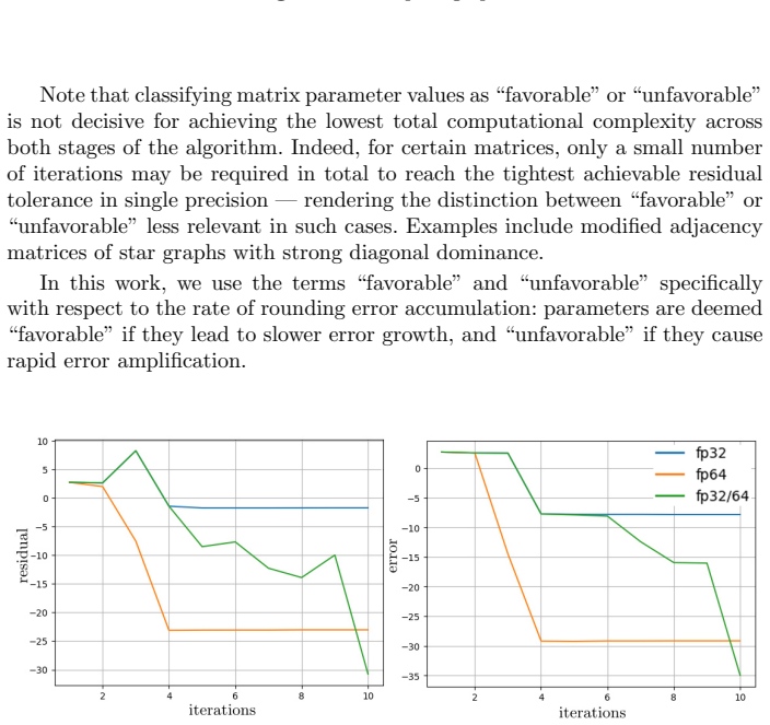

Figures from the paper (2 more)


Reference graph
Works this paper leans on
-
[1]
Higham, N.J., Mary, T.:Mixed precision algorithms in numerical linear algebra// Acta Numerica, v. 31, 347–414 (2022)
work page 2022
-
[2]
Abdelfattah, A., Anzt, H., Boman, E.G., Carson, E., Cojean, T., Dongarra, J., Fox, A., Gates, M., Higham, N.J., Li, X.S., Loe, J., Luszczek, P., Pranesh, S., Raja- manickam, S., Ribizel, T., Smith, B.F., Swirydowicz, K., Thomas, S., Tomov, S., Tsai, Y.M. and Yang, U.M.:A survey of numerical linear algebra methods utilizing mixed-precision arithmetic// Int...
work page 2021
-
[3]
Turner, K., Walker, H.F.:Efficient high accuracy solutions with GMRES(m)// SIAM J. Sci. Statist. Comput. 12, 815–825 (1992)
work page 1992
-
[4]
Nichols et al., eds), Springer, pp
Lindquist, N., Luszczek, P., Dongarra, J.:Improving the performance of the GM- RES method using mixed-precision techniques// Communications in Computer and Information Science (J. Nichols et al., eds), Springer, pp. 51–66 (2020)
work page 2020
-
[5]
Giraud, L., Haidar, A., Watson, L.T.:Mixed-precision preconditioners in parallel domain decomposition solvers// Domain Decomposition Methods in Science and Engineering XVII (U. Langer et al., eds), Vol. 60 of Lecture Notes in Computational Science and Engineering, Springer, 357–364 (2008)
work page 2008
-
[6]
Gratton, S., Simon, E., Titley-Peloquin, D., Toint, P.:Exploiting variable precision in GMRESAvailable at arXiv:1907.10550. (2019)
work page Pith review arXiv 2019
-
[7]
Aliaga, J.I., Anzt, H., Grutzmacher, T., Quintana-Orti, E.S., Tomas, A.E.:Com- pressed basis GMRES on high performance GPUsAvailable at arXiv:2009.12101. (2020)
work page Pith review arXiv 2020
-
[8]
Iterative Methods for Sparse Linear Systems
Saad, Y. Iterative Methods for Sparse Linear Systems. 2nd ed. Philadelphia: SIAM, 2003
work page 2003
Show all 23 references
-
[9]
Iterative Methods for Solving Linear Systems
Greenbaum, A. Iterative Methods for Solving Linear Systems. Philadelphia: SIAM, 1997. XXXV
1997
-
[10]
Simoncini, V., Szyld, D. B. Recent computational developments in Krylov subspace methods for linear systems // Numer. Linear Algebra Appl. Vol. 14, no. 1, 1–59 (2007)
2007
-
[11]
S., Noailles, J., Ruiz, D
Arioli, M., Duff, I. S., Noailles, J., Ruiz, D. A block projection method for sparse symmetric indefinite linear systems // SIAM J. Sci. Statist. Comput. Vol. 13, no. 2, 478–498 (1992)
1992
-
[12]
Fine-grained parallel incomplete LU factorization // SIAM J
Chow, E., Patel, A. Fine-grained parallel incomplete LU factorization // SIAM J. Sci. Comput. Vol. 37, no. 2. C169–C193 (2015)
2015
-
[13]
and Tuma, M.Preconditioning of linear least squares by robust incom- plete factorization for implicitly held normal equations// ACM Transactions on Mathematical Software, Vol
Scott, J. and Tuma, M.Preconditioning of linear least squares by robust incom- plete factorization for implicitly held normal equations// ACM Transactions on Mathematical Software, Vol. 42, no. 4, pp. 1–24 (2016)
2016
-
[14]
Carson, E., Higham, N. J. A new analysis of iterative refinement and its application to accurate solution of ill-conditioned sparse linear systems // SIAM J. Sci. Comput. Vol. 39, no. 6. A2834–A2856 (2017)
2017
-
[15]
Yang, S. et al. Mixed-precision iterative refinement with sparse approximate in- verses // arXiv preprint arXiv:2205.12345 (2022)
2022 arXiv
-
[16]
Conference MOTOR-2024 Challenges
Parameter optimization for restarted mixed precision it- erative sparse solver. Conference MOTOR-2024 Challenges. https://motor24.oscsbras.ru/challenges/Challenge3.pdf
2024
-
[17]
Burkhardt, P.: Optimal algebraic breadth-first search for sparse graphs // ACM Transactions on Knowledge Discovery from Data (TKDD), Volume 15, Issue 5 Ar- ticle No.: 77, 1–19. https://doi.org/10.1145/3446216 XXXVI Appendix 11 Samples used in the experiments 11.1 Samples of ex...
-
[18]
the kNN parameter takes five values:k∈ {1,5,10,15,20}. OnceN S is determined, the test sample size is defined as NT =N−N S , so thatT=S 0 \ S; that is, all matrices of a given type and size not selected for training are assigned to the test set. Consequently, the training set ...
-
[19]
the sizeN=|S 0|of the general sample, along with the sizesN S =|S|and NT =|T |of the training and test samples
-
[20]
The distribution of matrices by optimal tolerance ˆε 1: each entry in rowP and column ˆε1 gives the proportionP(as a percentage) of matrices inS 0 for which the optimal tolerance equals the column’s ˆε1; 3)k CG: the average number of CG iterations (over all matrices inS 0) whe...
-
[21]
classification accuracyAccof the kNN classifier used inAlgorithm II
-
[22]
localization measureLocof feature vectors (defined as the average fraction of same-class neighbors among theknearest neighbors)
-
[23]
All reported values are expressed as percentages
efficiencyEofAlgorithm IIrelative to full double-precision CG, reported for two choices ofω: fixed (ω= 1/3) and adaptive (ω=t sp/tdp). All reported values are expressed as percentages. Columns prefixed withM (e.g.,MAcc) denote mean values, while those prefixed withσ(e.g.,σAcc)...
Reviewed August 11, 2026 · model on record in the stance chip above.
Discussion (0). Continue with ORCID to comment.