REVIEW 2 major objections 5 minor 24 references
Numerical upscaling of perturbed diffusion problems
T0 review · 2 major / 5 minor · reviewed 2026-08-14 · deepseek-v4-flash
Pith's one-line read The paper establishes that perturbed diffusion problems can be solved by reusing reference-coefficient computations wherever local error indicators are small, with a global error bound that preserves the multiscale convergence order.
desk verdict Useful extension of PG-LOD for perturbed coefficients with a sound core analysis, but the printed algorithm does not match the analyzed method and as written cannot reproduce the experiments—fixable, but essential. read the letter →
The pith
A machine-rendered reading of the paper's core claim, the machinery that carries it, and where it could break.
The reading
What carries the argument
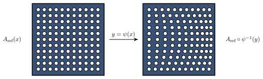
The load-bearing object is the localized corrector pair $(Q_{k,T},R_{k,T})$ of the PG-LOD method: for each coarse element $T$, these solve fine-scale patch problems with the perturbed coefficient, and the corresponding reference objects $(Q^{\mathrm{ref}}_{k,T},R^{\mathrm{ref}}_{k,T})$ are precomputed once. The mechanism that makes reuse safe is the set of error indicators (3.9), written in terms of $\delta=A^{-1/2}(A-A_{\mathrm{ref}})A_{\mathrm{ref}}^{-1/2}$ and precomputable coarse quantities such as the eigenvalue ratios $\tilde\mu_{T,T'}$ of (5.1). Lemma 4.2 shows each indicator controls the true difference between perturbed and reference correctors, and Theorem 4.1 converts the summed indicator errors, together with the exponential localization error $k^{d/2}\theta^k$, into the global bound. The domain-mapping representation $A=\det(J)J^{-1}(A_{\mathrm{ref}}-D)J^{-T}$ is what turns a geometric shift of the material into a value perturbation of the reference coefficient, which is the form the indicators can see.
What would settle it
Refine the coarse mesh and compute, on an element next to a fixed defect, the true local corrector error $|||Q_{k,T}v-Q^{\mathrm{ref}}_{k,T}v|||$ alongside the indicator $E_{QV_H,T}$; if their ratio is unbounded as $H\to0$, Lemma 4.2 fails and Theorem 4.1 collapses. A reader could run this local test because the paper reports only the global relative error, not the indicator-to-error ratio.
Extended reading notes
Core claim
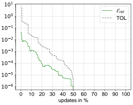
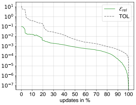
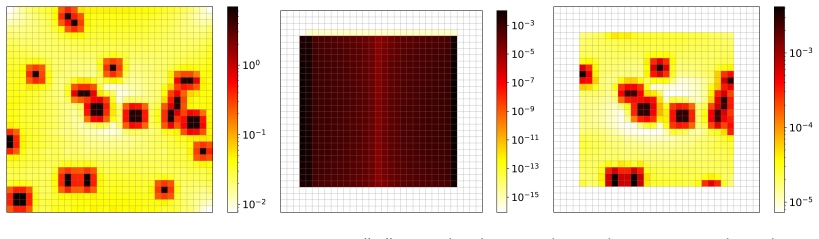
The authors claim that reference-coefficient computations can be recycled safely in an adaptive multiscale solver. In precise terms, Theorem 4.1 states that when the error indicators of (3.10) are below a tolerance with $\mathrm{TOL}=\tau k^{-d/2}$, the solution $\tilde u_k$ produced by mixing reference and perturbed correctors obeys $|||u-\tilde u_k||| \lesssim k^{d/2}(\theta^k+\mathrm{TOL})(\|f\|_{L^2(\Omega)}+|||g|||)$, with constants independent of $H$, $k$, $\tau$, and $\mathrm{TOL}$. The proof bounds each local corrector error by a computable indicator (Lemma 4.2) and then shows that the mixed bilinear form remains coercive, so the adaptive update contributes only a term proportional to the tolerance. The numerical experiments show that local defects are detected sharply by the indicators and that the error decreases quickly with the percentage of updated correctors; a global domain mapping is the hard case, where many elements are marked. The intended conclusion is that for the right perturbation classes, the method achieves near full-recomputation accuracy while updating only a small fraction of the local problems.
Load-bearing premise
The savings rest on the premise that a large fraction of coarse elements can be marked safe by the local error indicators; if the perturbation is large everywhere or does not fit the defect-plus-coordinate-change representation, nearly every element must be recomputed and the method degenerates to full recomputation.
Editorial extensions
If this is right
- If the marking criterion (3.10) is met, the adaptive PG-LOD solution has the same order of accuracy as a full recomputation up to the TOL term, so the reuse is theoretically safe rather than heuristic.
- For local defects, the indicators concentrate around the defect and decay exponentially away from it, so most coarse elements keep their reference correctors and the cost per perturbed solve is dominated by a coarse-scale system plus a few local patches.
- The reference stage stores only coarse-scale data of size $k^d H^{-d}$ and can be parallelized over elements; each perturbed solve is then independent, so many perturbations can be processed in parallel with low communication.
- Global domain mappings are the limiting case: the marked fraction grows, and the reuse advantage shrinks, although the method still converges; for a completely changed coefficient without a mapping, the approach reduces to recomputation.
- Periodic reference structures allow corrector reuse across periodic patches, further reducing memory and complexity.
Reading between the lines
- Editorial extension: the same indicator-driven reuse could be applied to sequences of coefficients that drift slowly in time, with the reference stage refreshed only when the marked fraction grows, yielding per-time-step cost proportional to the amount of coefficient change instead of the full problem.
- Editorial extension: the eigenvalue precomputation of $\tilde\mu_{T,T'}$ suggests a practical screening tool, where after a manufactured sample is measured only the per-element coefficient deviation $\|\delta\|_{L^\infty}$ is needed to decide which regions require new simulations.
- Editorial extension: perturbations that change the topology of the high-conductivity phase are not naturally captured by the defect-plus-mapping form, and the indicators would likely mark a large fraction of elements; representing such perturbations would require a different parametrization or periodic reference updates.
Signed reviews
Editorial analysis
A structured set of objections, weighed in public.
Referee Report
Summary. The manuscript proposes an adaptive Petrov--Galerkin localized orthogonal decomposition (PG-LOD) method for elliptic diffusion problems whose coefficient is a perturbation of a reference coefficient. The perturbations considered are local defects and global or local domain mappings, possibly combined. The method precomputes reference correctors and element stiffness contributions, computes four local error indicators for each coarse element, and then decides adaptively which elements need recomputation of correctors using the perturbed data. The central theoretical result, Theorem 4.1, states an error bound of the form |||u - \tilde u_k||| ≲ k^{d/2}(θ^k + TOL)(||f||_{L^2(Ω)} + |||g|||) under the marking conditions in Definition 3.5. Numerical experiments for random defects, local domain mappings, and a global domain mapping are reported, together with reproducibility information for the implementation. The main technical framework is standard LOD machinery combined with perturbation indicators, and the paper is generally well organized; however, the printed Algorithm 1 does not implement the analyzed method, and the proof of Theorem 4.1 contains a flawed norm estimate that needs correction.
Significance. If the implementation and proof are corrected, the paper would be a useful contribution to multiscale simulation for parametric or perturbed coefficients. The idea of reusing reference-coefficient correctors and element matrices, with computable indicators that trigger local recomputation, is natural and practically relevant. The paper gives explicit indicator definitions, a parameter-free (up to standard LOD constants) theoretical bound, and numerical evidence for three perturbation regimes. The claim that local defects and mild domain mappings can be handled without recomputing the complete multiscale basis is credible and of interest to the LOD community. Credit is due for shipping reproducible code and for reporting the expected degradation in the global-mapping example rather than overclaiming efficiency. The main reservation is not the novelty but the consistency between the analysis and the algorithm as printed.
major comments (2)
- [Section 5.2, Algorithm 1 (lines 11–16)] As printed, Algorithm 1 does not implement the analyzed method. The marking condition in line 11 is max(E_QVH,T (||f||_{L2(T)} + |||g|||), E_f,T, E_Rf,T, E_Qg,T) ≤ TOL, which differs from the marking criterion (3.10) in several load-bearing ways: it does not sum E_f,T and E_Rf,T, it uses the local norm ||f||_{L2(T)} instead of the global norm ||f||_{L2(Ω)}, and it does not scale the right-hand side by ||f||_{L2(Ω)} + |||g|||. Therefore an element can be marked for reference reuse even when E_f,T + E_Rf,T > TOL(||f||_{L2(Ω)} + |||g|||), so the hypothesis of Theorem 4.1 need not hold for the algorithm. Moreover, lines 13–14 compute the perturbed correctors and the perturbed element matrix b_T for the elements T that have just been added to T_ref^H, while line 16 assembles b^ref_T for T ∈ T_ref^H and b_T for T ∉ T_ref^H. Thus b_T is computed exactly for the elements where it is not used and is never computed for the elements where the assembly requires it. As written, the algorithm cannot assemble the matrix in line 16. This inconsistency must be repaired, for example by moving the computation of b_T into an else-branch for T ∉ T_ref^H and by making the marking rule identical to (3.10).
- [Section 4, Eq. (4.3)] The displayed estimate for |||u_k - \tilde u_k||| in the proof of Theorem 4.1 contains sign errors. A norm satisfies the triangle inequality, so the terms -|||Q_k g - \tilde Q_k g||| (and the analogous negative signs in the following line) should be plus signs. In addition, bounding |||Q_k u^H_k - \tilde Q_k \tilde u^H_k||| requires inserting ±\tilde Q_k u^H_k and then using the boundedness of \tilde Q_k that is established just before (4.3); as written, the second line of (4.3) omits this step. Since (4.3) is the estimate that connects the reuse error to the coarse-scale error u^H_k - \tilde u^H_k, the proof of Theorem 4.1 needs this corrected calculation before the main bound can be considered established.
minor comments (5)
- [Section 4, Theorem 4.1 vs. Definition 3.5] The hypothesis of Theorem 4.1 is written in a different normalization from the marking criterion (3.10): the first term is multiplied by ||f||_{L2(Ω)} + |||g||| while the other two are not. The two statements are equivalent for nonzero data, but unifying the notation would prevent exactly the kind of mismatch that occurs in Algorithm 1.
- [Section 2.1 and Section 6.3] The text says that the global domain mapping experiment would surely result in 100% recomputation without domain mappings; this is a heuristic observation. Consider stating it as a comparison of indicator values rather than as a categorical claim, since the computational cost of the alternative is not measured in the experiment.
- [References] References [13] and [14] are the same paper and should be merged or one removed.
- [Abstract and Introduction] There are several typos, including 'communcation', 'mapppings', and 'performed'; the abstract and introduction should be proofread.
- [Algorithm 1] The indentation and block structure of Algorithm 1 is ambiguous: it should be made explicit whether the assembly in line 16 is inside or outside the loop over elements, and which 'end' closes the for loop.
Circularity Check
No circularity: Theorem 4.1 is proved from published LOD estimates and directly proven indicator bounds; the Algorithm 1 discrepancy is a consistency defect, not circularity.
full rationale
The paper's load-bearing analysis is self-contained. Theorem 4.1 is proved from three ingredients: the localization error bound (3.8) taken from the published PG-LOD theory ([12], [20]), the assumption that the marking criteria (3.10) hold, and Lemma 4.2, which is proved in the paper. Lemma 4.2 shows by direct energy estimates that the computable indicators E_QVH,T, E_f,T, E_Rf,T, and E_Qg,T dominate the corresponding corrector errors, and the theorem then sums these bounds over the marked set T^ref_H with the patch-overlap factor k^d. No step uses the numerical experiments to define a constant in the theorem, and no step fits TOL or the target solution. The use of [12] is a standard dependency: it supplies the PG-LOD framework and a parameter-free localization estimate whose assumptions do not include the theorem being proved in this paper. The numerical estimator ν_T ≤ 0.25H in Section 5.1 is calibrated on mesh-refinement problems for a local Poincare-type supremum, not on the target perturbed solutions, and it affects only the computable indicators, not the theoretical bound. The reviewer-observed discrepancy between Algorithm 1's marking rule (line 11) and Definition 3.5's rule (3.10), and the assembly of b_T for marked instead of unmarked elements, is a real correctness or consistency defect in the printed pseudocode, but it is not circularity: it does not make the theorem's derivation depend on its conclusion. No circular step can be exhibited, so the circularity score is 0.
Assumptions & free parameters
free parameters (3)
- TOL (marking tolerance) =
scanned from infinity (no updates) to 0 (all updates) in the experiments
- k (localization patch size) =
4 in all experiments
- nu_T coefficient =
0.25H
assumptions (5)
- standard math The interpolation operator IH satisfies the stability bound (3.1) on the quasi-uniform mesh.
- standard math Corrector operators decay exponentially with rate theta < 1 independent of H, k, and TOL ((3.7)).
- domain assumption The perturbed coefficient A = det(J)J^{-1}(Aref-D)J^{-T} is symmetric positive definite and uniformly elliptic, and J and J^{-1} are bounded a.e. with psi mapping the boundary to itself.
- domain assumption The fine mesh Th resolves the coefficient variations, and the analysis measures error relative to the discrete solution in Vh.
- domain assumption Bilinear isoparametric mappings psi are adequate for the domain mapping step.
Cite this review
Pith. "Pith review of Numerical upscaling of perturbed diffusion problems." pith.science (2026). https://pith.science/paper/KHUAS6L5
@misc{pith2026190800652,
  author       = {Pith},
  title        = {Pith review of: Numerical upscaling of perturbed diffusion problems},
  year         = {2026},
  howpublished = {\url{https://pith.science/paper/KHUAS6L5}},
  note         = {Machine review of arXiv:1908.00652}
}
read the original abstract
In this paper we study elliptic partial differential equations with rapidly varying diffusion coefficient that can be represented as a perturbation of a reference coefficient. We develop a numerical method for efficiently solving multiple perturbed problems by reusing local computations performed with the reference coefficient. The proposed method is based on the Petrov--Galerkin Localized Orthogonal Decomposition (PG-LOD) which allows for straightforward parallelization with low communcation overhead and memory consumption. We focus on two types of perturbations: local defects which we treat by recomputation of multiscale shape functions and global mappings of a reference coefficient for which we apply the domain mapping method. We analyze the proposed method for these problem classes and present several numerical examples.
Figures

Figures from the paper (5 more)


Reference graph
Works this paper leans on
-
[1]
Ivo Babuska and Robert Lipton. Optimal local approximation spaces for generalized finite element methods with application to multiscale problems.Multiscale Modeling & Simulation, 9(1):373–406, 2011
work page 2011
-
[2]
The mathematical theory of finite element methods , volume 15
Susanne Brenner and Ridgway Scott. The mathematical theory of finite element methods , volume 15. Springer Science & Business Media, 2007
work page 2007
-
[3]
Analytic regularity and collocation approximation for elliptic pdes with random domain deformations
Julio E Castrillon-Candas, Fabio Nobile, and Raul F Tempone. Analytic regularity and collocation approximation for elliptic pdes with random domain deformations. Computers & Mathematics with Applications , 71(6):1173–1197, 2016. 21
work page 2016
-
[4]
Philippe G Ciarlet and Pierre-Arnaud Raviart. The combined effect of curved boundaries and numerical integration in isoparametric finite element methods. In The mathematical foundations of the finite element method with applications to partial differential equations , pages 409–474. Elsevier, 1972
work page 1972
-
[5]
On multiscale methods in petrov– galerkin formulation
Daniel Elfverson, Victor Ginting, and Patrick Henning. On multiscale methods in petrov– galerkin formulation. Numerische Mathematik, 131(4):643–682, 2015
work page 2015
-
[6]
Efficient imple- mentation of the localized orthogonal decomposition method
Christian Engwer, Patrick Henning, Axel M˚ alqvist, and Daniel Peterseim. Efficient imple- mentation of the localized orthogonal decomposition method. Computer Methods in Applied Mechanics and Engineering, 2019
work page 2019
-
[7]
Stable multiscale petrov–galerkin finite element method for high frequency acoustic scattering
Dietmar Gallistl and Daniel Peterseim. Stable multiscale petrov–galerkin finite element method for high frequency acoustic scattering. Computer Methods in Applied Mechanics and Engineering, 295:1–17, 2015
work page 2015
-
[8]
Analysis of the domain map- ping method for elliptic diffusion problems on random domains
Helmut Harbrecht, Michael Peters, and Markus Siebenmorgen. Analysis of the domain map- ping method for elliptic diffusion problems on random domains. Numerische Mathematik , 134(4):823–856, 2016
work page 2016
Show all 24 references
-
[9]
Fredrik Hellman and Tim Keil. gridlod. https://github.com/fredrikhellman/gridlod
-
[10]
gridlod-on-perturbations-super
Fredrik Hellman and Tim Keil. gridlod-on-perturbations-super. https://github.com/ gridlod-community/gridlod-on-perturbations-super
-
[11]
Contrast independent localization of multiscale prob- lems
Fredrik Hellman and Axel M˚ alqvist. Contrast independent localization of multiscale prob- lems. Multiscale Modeling & Simulation , 15(4):1325–1355, 2017
2017
-
[12]
Numerical homogenization of elliptic pdes with similar coefficients
Fredrik Hellman and Axel M˚ alqvist. Numerical homogenization of elliptic pdes with similar coefficients. Multiscale Modeling & Simulation , 17(2):650–674, 2019
2019
-
[14]
Localized orthogonal decomposition techniques for boundary value problems
Patrick Henning and Axel M˚ alqvist. Localized orthogonal decomposition techniques for boundary value problems. SIAM Journal on Scientific Computing , 36(4):A1609–A1634, 2014
2014
-
[15]
A multiscale finite element method for elliptic problems in composite materials and porous media
Thomas Y Hou and Xiao-Hui Wu. A multiscale finite element method for elliptic problems in composite materials and porous media. Journal of computational physics, 134(1):169–189, 1997
1997
-
[16]
The varia- tional multiscale method—a paradigm for computational mechanics
Thomas JR Hughes, Gonzalo R Feij´ oo, Luca Mazzei, and Jean-Baptiste Quincy. The varia- tional multiscale method—a paradigm for computational mechanics. Computer methods in applied mechanics and engineering , 166(1-2):3–24, 1998
1998
-
[17]
Variational crimes in the localized orthogonal decomposition method, 2018
Tim Keil. Variational crimes in the localized orthogonal decomposition method, 2018
2018
-
[18]
Some numerical approaches for weakly random homogenization
Claude Le Bris. Some numerical approaches for weakly random homogenization. In Numer- ical mathematics and advanced applications 2009 , pages 29–45. Springer, 2010
2009
-
[19]
Multiscale finite element approach for “weakly” random problems and related issues
Claude Le Bris, Fr´ ed´ eric Legoll, and Florian Thomines. Multiscale finite element approach for “weakly” random problems and related issues. ESAIM: Mathematical Modelling and Numerical Analysis, 48(3):815–858, 2014. 22
2014
-
[20]
Localization of elliptic multiscale problems
Axel M˚ alqvist and Daniel Peterseim. Localization of elliptic multiscale problems. Mathe- matics of Computation , 83(290):2583–2603, 2014
2014
-
[21]
Computation of eigenvalues by numerical upscaling
Axel M˚ alqvist and Daniel Peterseim. Computation of eigenvalues by numerical upscaling. Numerische Mathematik, 130(2):337–361, 2015
2015
-
[22]
Gamblets for opening the complexity-bottleneck of im- plicit schemes for hyperbolic and parabolic odes/pdes with rough coefficients
Houman Owhadi and Lei Zhang. Gamblets for opening the complexity-bottleneck of im- plicit schemes for hyperbolic and parabolic odes/pdes with rough coefficients. Journal of Computational Physics, 347:99–128, 2017
2017
-
[23]
Variational multiscale stabilization and the exponential decay of fine- scale correctors
Daniel Peterseim. Variational multiscale stabilization and the exponential decay of fine- scale correctors. In Building bridges: connections and challenges in modern approaches to numerical partial differential equations, pages 343–369. Springer, 2016
2016
-
[24]
Robust numerical upscaling of elliptic multiscale problems at high contrast
Daniel Peterseim and Robert Scheichl. Robust numerical upscaling of elliptic multiscale problems at high contrast. Computational Methods in Applied Mathematics , 16(4):579–603, 2016
2016
-
[25]
Heterogeneous multiscale method: a general methodology for multiscale modeling
E Weinan, Bj¨ orn Engquist, and Zhongyi Huang. Heterogeneous multiscale method: a general methodology for multiscale modeling. Physical Review B, 67(9):092101, 2003. 23
2003
Reviewed August 14, 2026 · model on record in the stance chip above.
Discussion (0). Continue with ORCID to comment.