REVIEW 2 major objections 1 minor 1 cited by
End-to-end optimization of subgrid scale models for discontinuous spectral element schemes based on the discrete adjoint method
T0 review · 2 major / 1 minor · reviewed 2026-06-28 · grok-4.3
Pith's one-line read A discrete adjoint framework optimizes subgrid-scale model parameters inside a spectral difference LES solver.
desk verdict The paper gives a working discrete-adjoint loop for tuning SGS parameters inside a spectral-difference solver, but the Legendre-mode decay objective leaves open whether the gains are physically meaningful or just damping artifacts. read the letter →
The pith
A machine-rendered reading of the paper's core claim, the machinery that carries it, and where it could break.
The reading
What carries the argument
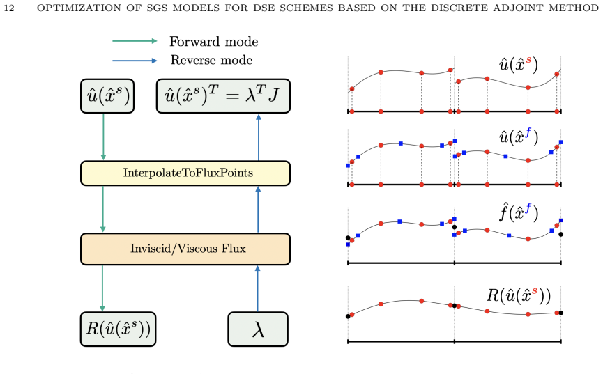
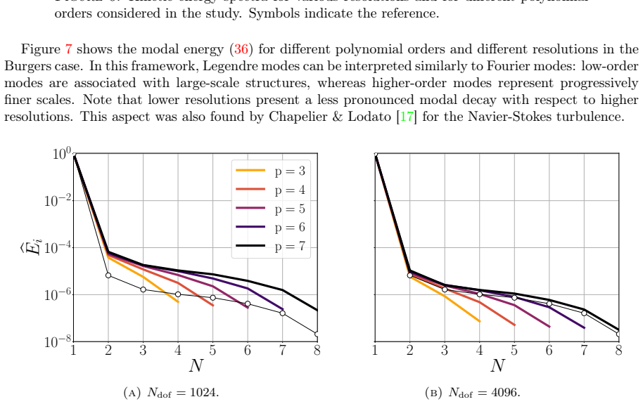
The discrete adjoint method applied to the Spectral Difference scheme, with the objective function defined as the spatio-temporally averaged decay of Legendre modal coefficients.
What would settle it
An independent test case in which the optimized SGS model produces larger errors than the baseline model in key turbulence statistics would falsify the improvement claim.
Extended reading notes
Core claim
The central claim is that optimizing a limited set of parameters in classical and nonlinear SGS models through a discrete adjoint framework inside the SD discretization produces models that achieve significant improvements over baseline closures in forced and decaying homogeneous isotropic turbulence as well as the Taylor-Green vortex, with robustness across resolutions, polynomial orders, and Reynolds numbers.
Load-bearing premise
The spatio-temporally averaged decay of the Legendre modal coefficients provides a suitable and stable objective function for the optimization in chaotic LES systems.
Editorial extensions
If this is right
- The optimized SGS models generalize to out-of-sample flow configurations including decaying homogeneous isotropic turbulence and the Taylor-Green vortex.
- Performance gains hold across variations in grid resolution, polynomial order, and Reynolds number.
- Both the Smagorinsky model and non-linear tensor-basis formulations benefit from the parameter optimization.
- The methodology applies to both one-dimensional Burgers turbulence and three-dimensional cases.
Reading between the lines
- The framework could extend to other high-order discontinuous methods for turbulence modeling.
- Different objective functions might further improve optimization stability in other chaotic flow regimes.
- Such tuned models could reduce the need for manual calibration when applying LES to engineering flows.
Editorial analysis
A structured set of objections, weighed in public.
Referee Report
Summary. The manuscript develops a discrete-adjoint optimization framework, leveraging automatic differentiation in a high-order Spectral Difference solver, to calibrate parameters of classical SGS models (Smagorinsky and nonlinear tensor-basis forms) against filtered DNS data. The objective is the spatio-temporally averaged decay rate of Legendre modal coefficients; optimization is performed on forced HIT at varying resolutions and polynomial orders, with out-of-sample assessment on decaying HIT and Taylor-Green vortex. The central claim is that the resulting models yield significant improvements over baseline closures in all tested configurations.
Significance. If the central claim holds, the work offers a systematic route to SGS-model calibration that accounts for the interaction with a specific high-order discretization, which is a recognized challenge in LES. The explicit use of the discrete adjoint for end-to-end optimization in chaotic turbulent flows is a methodological strength that could be adopted more broadly if the chosen objective is shown to produce physically consistent models.
major comments (2)
- [objective-function paragraph] The paragraph describing the objective function (abstract and methods): the manuscript asserts that the spatio-temporally averaged decay of Legendre modal coefficients is a suitable and stable objective for chaotic LES optimization, yet provides no demonstration that minimization of this scalar produces correct inter-scale energy transfer, kinetic-energy spectra, or dissipation rates on the out-of-sample DHIT and Taylor-Green cases. If the functional primarily damps high-mode energy without enforcing spectral shape, the reported improvements may be limited to the training objective and not generalize to physically relevant diagnostics.
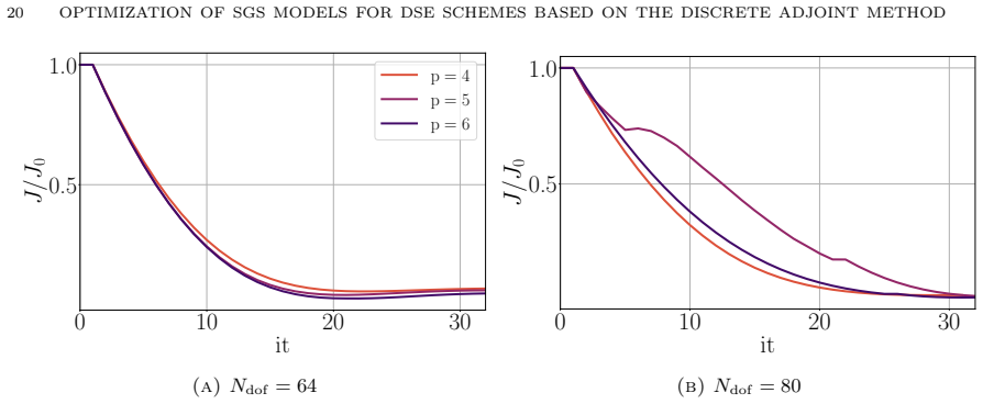
- [out-of-sample assessment] Results section on out-of-sample tests: the claim of 'significant improvements over baseline SGS closures' in all test cases is load-bearing for the central contribution, but the manuscript supplies no quantitative metrics (e.g., relative error reduction in spectra or structure functions, convergence histories of the adjoint optimization, or error bars across realizations). Without these data it is impossible to judge whether the improvements are robust or merely marginal.
minor comments (1)
- [methods] Notation for the modal-coefficient decay rate should be defined explicitly with an equation number rather than described only in prose.
Simulated Author's Rebuttal
We thank the referee for the constructive comments. We address each major comment below.
read point-by-point responses
-
Referee: [objective-function paragraph] The paragraph describing the objective function (abstract and methods): the manuscript asserts that the spatio-temporally averaged decay of Legendre modal coefficients is a suitable and stable objective for chaotic LES optimization, yet provides no demonstration that minimization of this scalar produces correct inter-scale energy transfer, kinetic-energy spectra, or dissipation rates on the out-of-sample DHIT and Taylor-Green cases. If the functional primarily damps high-mode energy without enforcing spectral shape, the reported improvements may be limited to the training objective and not generalize to physically relevant diagnostics.
Authors: The objective was selected because matching modal decay rates from filtered DNS directly encodes the correct inter-scale transfer for the SD discretization. We agree additional evidence is needed and will add kinetic-energy spectra, dissipation-rate comparisons, and inter-scale transfer diagnostics for the out-of-sample cases in the revision. revision: yes
-
Referee: [out-of-sample assessment] Results section on out-of-sample tests: the claim of 'significant improvements over baseline SGS closures' in all test cases is load-bearing for the central contribution, but the manuscript supplies no quantitative metrics (e.g., relative error reduction in spectra or structure functions, convergence histories of the adjoint optimization, or error bars across realizations). Without these data it is impossible to judge whether the improvements are robust or merely marginal.
Authors: We agree that quantitative support is required. The revised manuscript will report relative error reductions on spectra and structure functions, adjoint optimization convergence histories, and error bars from multiple realizations. revision: yes
Circularity Check
No significant circularity detected
full rationale
The paper optimizes a small set of SGS parameters by minimizing a modal-decay objective against filtered DNS data within a discrete-adjoint loop, then evaluates the resulting models on explicitly out-of-sample configurations (DHIT, Taylor-Green vortex) at varied resolutions and Reynolds numbers. No derivation step equates a claimed prediction to its own fitted inputs by construction, nor does any load-bearing premise rest on a self-citation chain; the reported improvements are therefore externally falsifiable and independent of the training data used for optimization.
Assumptions & free parameters
free parameters (1)
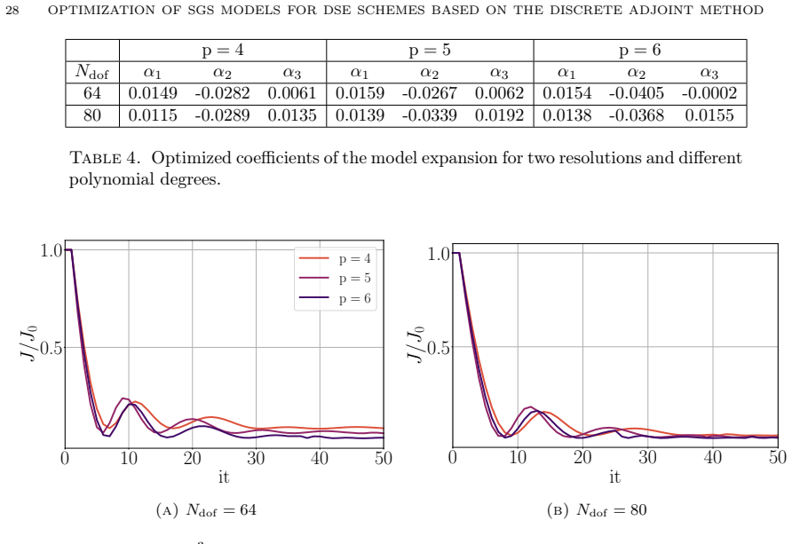
- SGS model parameters (Smagorinsky constant and nonlinear coefficients)
assumptions (1)
- domain assumption The spatio-temporally averaged decay of Legendre modal coefficients is an appropriate objective for chaotic turbulent flows.
Cite this review
Pith. "Pith review of End-to-end optimization of subgrid scale models for discontinuous spectral element schemes based on the discrete adjoint method." pith.science (2026). https://pith.science/paper/KIJQDDJS
@misc{pith2026260601150,
  author       = {Pith},
  title        = {Pith review of: End-to-end optimization of subgrid scale models for discontinuous spectral element schemes based on the discrete adjoint method},
  year         = {2026},
  howpublished = {\url{https://pith.science/paper/KIJQDDJS}},
  note         = {Machine review of arXiv:2606.01150}
}
read the original abstract
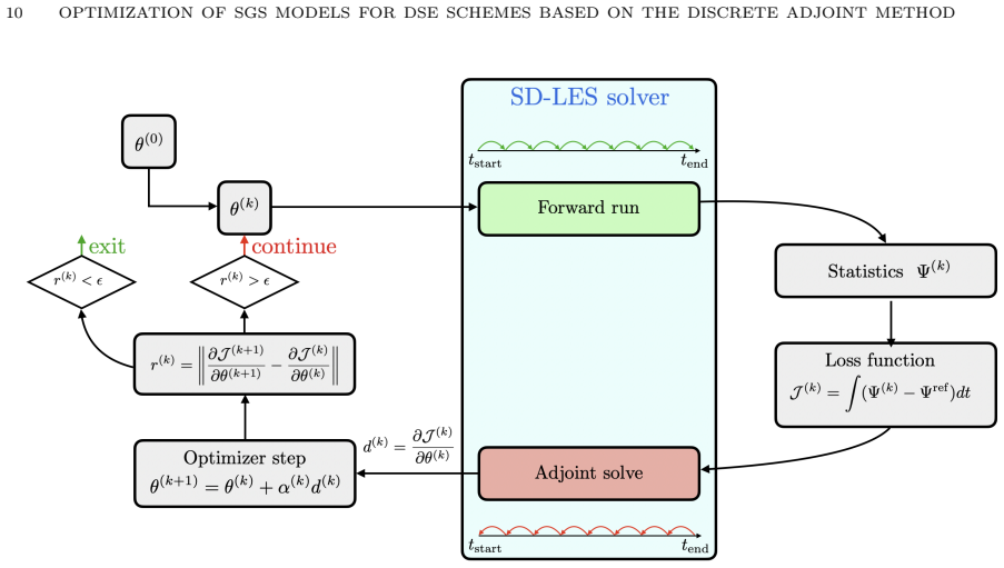
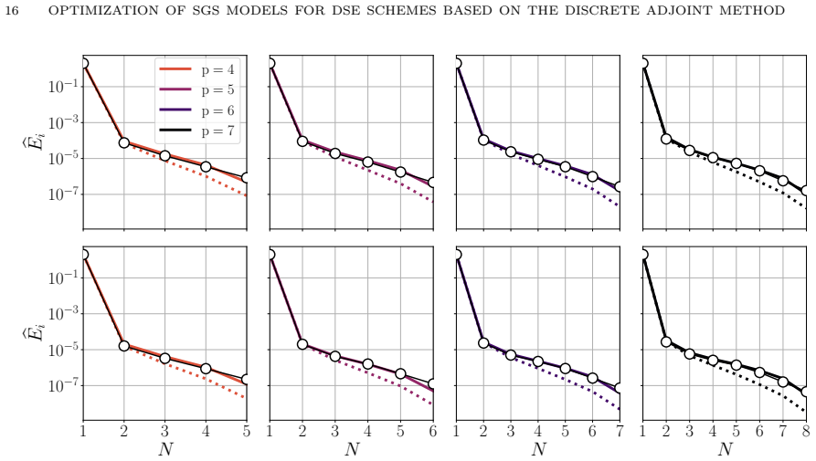
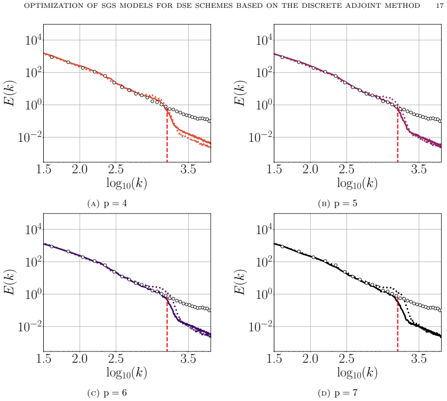
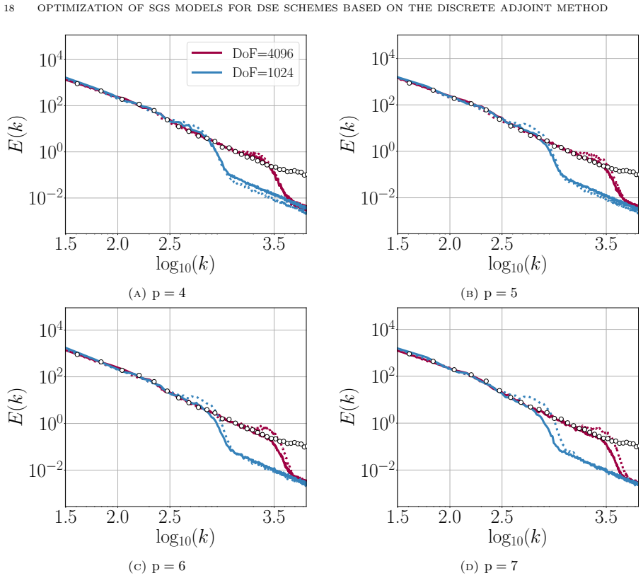
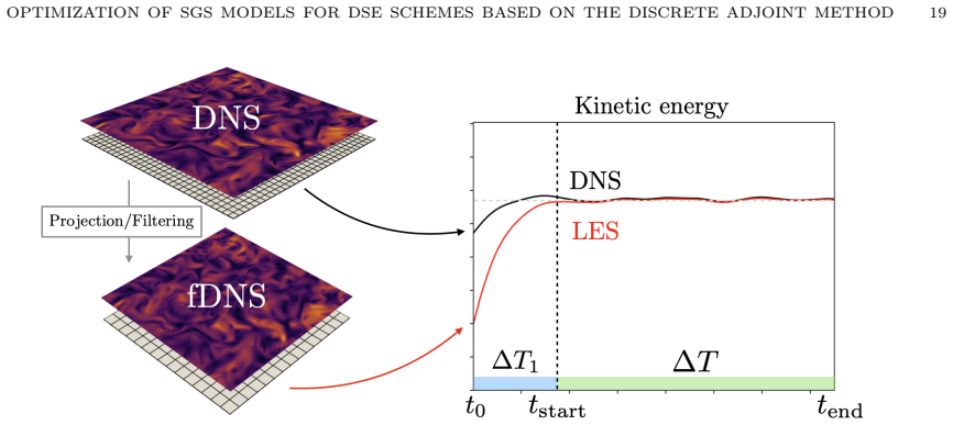
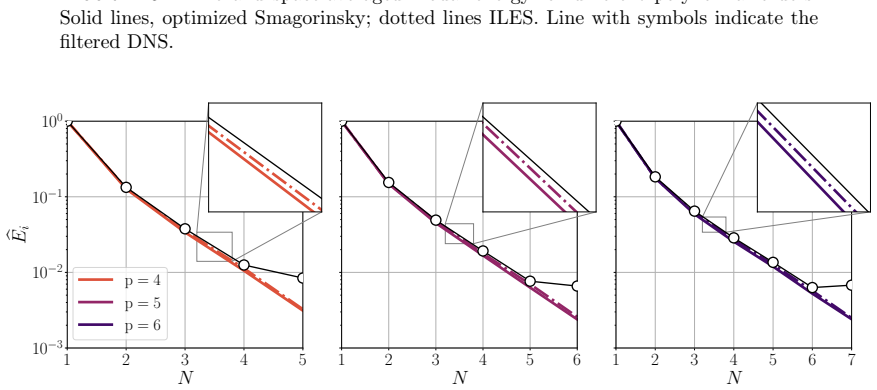
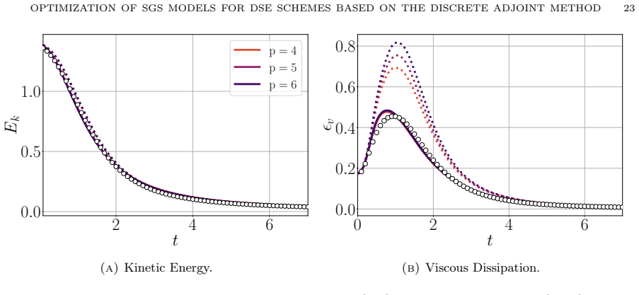
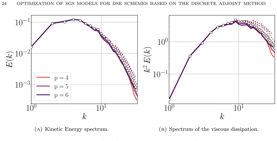
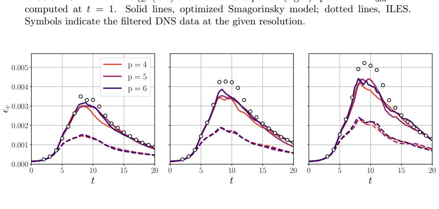
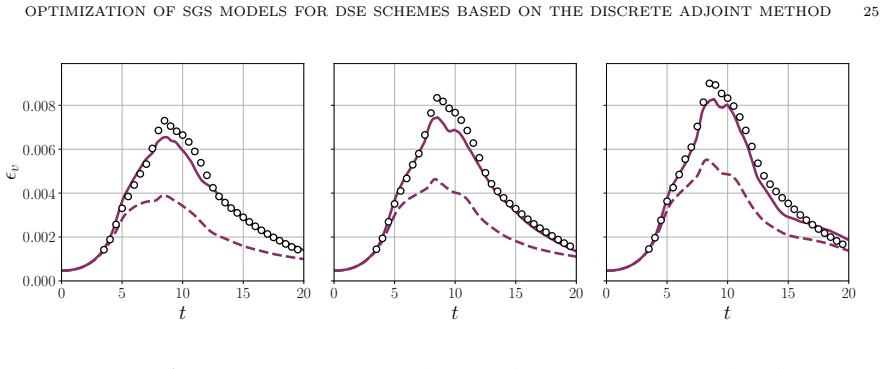
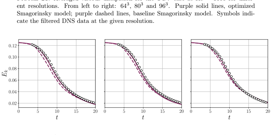
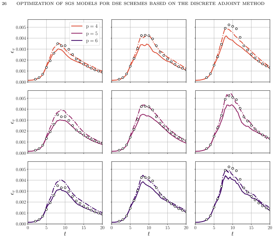
In computational fluid dynamics, Large Eddy Simulation (LES) offers a compelling balance between accuracy and computational cost by resolving large-scale flow structures while modeling unresolved subgrid scales. However, its predictive capacity is critically dependent on the choice and calibration of subgrid-scale (SGS) models, which often involve problem-dependent parameters and exhibit intricate interactions with the numerical discretization. In this work, we propose a discrete-adjoint framework to optimize SGS model parameters in the loop, leveraging automatic differentiation within a high-order Spectral Difference (SD) solver. Coarse-grained simulations of Forced Homogeneous Isotropic Turbulence (FHIT), together with filtered Direct Numerical Simulation (DNS) data, are used to optimize a limited set of parameters for classical SGS models, including the Smagorinsky model and non-linear tensor-basis formulations. For chaotic systems such as LES, the choice of objective function plays a crucial role in the stability and accuracy of the optimization. Here, we consider the spatio-temporally averaged decay of the Legendre modal coefficients as the quantity of interest for the SD scheme. The optimization is performed across different grid resolutions and polynomial orders, highlighting the impact of numerical discretization on model performance. The methodology is applied to both one-dimensional Burgers turbulence and fully three-dimensional turbulence. The trained models are subsequently assessed on out-of-sample configurations, including Decaying Homogeneous Isotropic Turbulence (DHIT) and the Taylor-Green vortex. Variations in polynomial order, grid resolution, and Reynolds number are considered to evaluate robustness and generalization. In all test cases, the optimized models demonstrate significant improvements over baseline SGS closures.
Figures
Figures from the paper (23 more)
Forward citations
Cited by 1 Pith paper
-
A novel compact scheme for second-order fluxes applied to the Spectral Difference method
A compact, parameter-free centered viscous flux for the Spectral Difference method reduces the diffusive stencil from five to three elements and restores optimal convergence at even polynomial orders.
Reference graph
Works this paper leans on
-
[1]
S. D. Agdestein and B. Sanderse. Discretize first, filter next: Learning divergence-consistent closure models for large-eddy simulation.Journal of Computational Physics, 522:113577, 2025
2025
-
[2]
S. D. Agdestein and B. Sanderse. A differentiable software suite for accelerated simulation of turbulent flows, 2026
2026
-
[3]
A. S. Ashley, J. Crean, and J. E. Hicken. Towards aerodynamic shape optimization of unsteady turbulent flows. In AIAA Scitech 2019 Forum, page 0168, 2019
2019
-
[4]
Balay, S
S. Balay, S. Abhyankar, M. F. Adams, S. Benson, J. Brown, P. Brune, K. Buschelman, E. M. Constantinescu, L. Dalcin, A. Dener, V. Eijkhout, J. Faibussowitsch, W. D. Gropp, V. Hapla, T. Isaac, P. Jolivet, D. Karpeev, D. Kaushik, M. G. Knepley, F. Kong, S. Kruger, D. A. May, L. C. McInnes, R. T. Mills, L. Mitchell, T. Munson, J. E. Roman, K. Rupp, P. Sanan, ...
2025
-
[5]
Bardina, J
J. Bardina, J. Ferziger, and W. Reynolds.Improved subgrid-scale models for large-eddy simulation
-
[6]
A. Beck, D. Flad, and C.-D. Munz. Deep neural networks for data-driven les closure models.Journal of Computational Physics, 398:108910, 2019
2019
-
[7]
A. Beck, G. Gassner, and C.-D. Munz. High order and underresolution. In R. Ansorge, H. Bijl, A. Meister, and T. Sonar, editors,Recent Developments in the Numerics of Nonlinear Hyperbolic Conservation Laws, volume 120 of Notes on Numerical Fluid Mechanics and Multidisciplinary Design, pages 41–55. Springer Berlin Heidelberg, 2013. Lectures Presented at a W...
2013
-
[8]
Beck and M
A. Beck and M. Kurz. Toward discretization-consistent closure schemes for large eddy simulation using reinforcement learning.Physics of Fluids, 35(12), 2023. OPTIMIZATION OF SGS MODELS FOR DSE SCHEMES BASED ON THE DISCRETE ADJOINT METHOD 31
2023
Show all 119 references
-
[9]
A. D. Beck, T. Bolemann, D. Flad, H. Frank, G. J. Gassner, F. Hindenlang, and C.-D. Munz. High-order discon- tinuous Galerkin spectral element methods for transitional and turbulent flow simulations.International Journal for Numerical Methods in Fluids, 76(8):522–548, 2014
2014
-
[10]
T. R. Bewley, P. Moin, and R. Temam. Dns-based predictive control of turbulence: an optimal benchmark for feedback algorithms.Journal of Fluid Mechanics, 447:179–225, 2001
2001
-
[11]
D. A. Bezgin, A. B. Buhendwa, and N. A. Adams. Jax-fluids 2.0: Towards hpc for differentiable cfd of compressible two-phase flows.Computer Physics Communications, 308:109433, 2025
2025
-
[12]
D. A. Bezgin, A. B. Buhendwa, S. J. Schmidt, and N. A. Adams. Ml-iles: End-to-end optimization of data-driven high-order godunov-type finite-volume schemes for compressible homogeneous isotropic turbulence.Journal of Com- putational Physics, 522:113560, 2025
2025
-
[13]
Biferale
L. Biferale. The decay of homogeneous anisotropic turbulence.Physics of Fluids, 15(8):2105–2112, 2003
2003
-
[14]
P.J.Blonigan.New methods for sensitivity analysis of chaotic dynamical systems.PhDthesis, MassachusettsInstitute of Technology, 2013
2013
-
[15]
Chapelier
J.-B. Chapelier. A coherent vorticity preserving eddy-viscosity correction for large-eddy simulation.Journal of Com- putational Physics, 359:164–182, 2018
2018
-
[17]
Chapelier and G
J.-B. Chapelier and G. Lodato. A spectral-element dynamic model for the large-eddy simulation of turbulent flows. Journal of Computational Physics, 321:279–302, 2016
2016
-
[18]
Chapelier and G
J.-B. Chapelier and G. Lodato. Optimal high-order spectral difference schemes for the computation of aeroacoustics and turbulence. In55th AIAA Aerospace Sciences Meeting, page 1228, 2017
2017
-
[19]
J. R. Chasnov. The decay of axisymmetric homogeneous turbulence.Physics of Fluids, 7(3):600–605, 03 1995
1995
-
[20]
F. K. Chow and P. Moin. A further study of numerical errors in Large-Eddy Simulations.Journal of Computational Physics, 184(2):366–380, 2003
2003
-
[21]
R. A. Clark, J. H. Ferziger, and W. C. Reynolds. Evaluation of subgrid-scale models using an accurately simulated turbulent flow.Journal of Fluid Mechanics, 91(1):1–16, 1979
1979
-
[22]
Clinco, N
N. Clinco, N. Tonicello, and G. Rozza. A data-driven study on implicit les using a spectral difference method.Journal of Computational Physics, 540:114302, 2025
2025
-
[23]
Cockburn and C
B. Cockburn and C. Shu. The local discontinuous Galerkin finite element method for convection-diffusion systems. SIAM Journal of Numerical Analysis, 35:2440–2463, 1998
1998
-
[24]
Cockburn and C
B. Cockburn and C. Shu. The Runge-Kutta discontinuous Galerkin finite element method for conservation laws V: Multidimensional systems.Journal of Computational Physics, 141:199–224, 1998
1998
-
[25]
M.deCrouy-Chanel, C.Mimeau, I.Mortazavi, A.Mariotti, andM.V.Salvetti.Large-eddysimulationswithremeshed vortex methods: An assessment and calibration of subgrid-scale models.Computers & Fluids, 277:106287, 2024
2024
-
[26]
de Laage de Meux, B
B. de Laage de Meux, B. Audebert, R. Manceau, and R. Perrin. Anisotropic linear forcing for synthetic turbulence generation in large eddy simulation and hybrid rans/les modeling.Physics of Fluids, 27(3):035115, 03 2015
2015
-
[27]
C. C. De Wiart, K. Hillewaert, L. Bricteux, and G. Winckelmans. Implicit les of free and wall-bounded turbulent flows based on the discontinuous galerkin/symmetric interior penalty method.International Journal for Numerical Methods in Fluids, 78(6):335–354, 2015
2015
-
[28]
Duraisamy, G
K. Duraisamy, G. Iaccarino, and H. Xiao. Turbulence modeling in the age of data.Annual Review of Fluid Mechanics, 51(Volume 51, 2019):357–377, 2019
2019
-
[29]
Fernandez, R
P. Fernandez, R. C. Moura, G. Mengaldo, and J. Peraire. Non-modal analysis of spectral element methods: Towards accurate and robust large-eddy simulations.Computer Methods in Applied Mechanics and Engineering, 346:43–62, 2019
2019
-
[30]
Fernandez, N.-C
P. Fernandez, N.-C. Nguyen, and J. Peraire. Subgrid-scale modeling and implicit numerical dissipation in dg-based large-eddy simulation. In23rd AIAA Computational Fluid Dynamics Conference, page 3951, 2017
2017
-
[31]
Fernandez, N.-C
P. Fernandez, N.-C. Nguyen, and J. Peraire. On the ability of Discontinuous Galerkin methods to simulate under- resolved turbulent flows. 2018
2018
-
[32]
Fernandez, N.-C
P. Fernandez, N.-C. Nguyen, and J. Peraire. On the ability of discontinuous Galerkin methods to simulate under- resolved turbulent flows.arXiv preprint arXiv:1810.09435, 2018
2018 arXiv
-
[33]
Garnier, N
E. Garnier, N. A. Adams, and P. Sagaut.Large-Eddy Simulation for compressible flows, volume 276. Springer, 2009
2009
-
[34]
Gassner and D
G. Gassner and D. A. Kopriva. A comparison of the dispersion and dissipation errors of gauss and gauss–lobatto discontinuous galerkin spectral element methods.SIAM Journal on Scientific Computing, 33(5):2560–2579, 2011
2011
-
[35]
Germano, U
M. Germano, U. Piomelli, P. Moin, and W. H. Cabot. A dynamic subgrid-scale eddy viscosity model.Physics of fluids A: Fluid dynamics, 3(7):1760–1765, 1991
1991
-
[36]
Ghiasi, J
Z. Ghiasi, J. Komperda, D. Li, A. Peyvan, D. Nicholls, and F. Mashayek. Modal explicit filtering for Large Eddy simulation in discontinuous spectral element method.Journal of Computational Physics: X, 3:100024, 2019
2019
-
[37]
S.Ghosal.AnanalysisofnumericalerrorsinLarge-Eddysimulationsofturbulence.Journal of Computational Physics, 125(1):187–206, 1996
1996
-
[38]
M. B. Giles and N. A. Pierce. An introduction to the adjoint approach to design.Flow, Turbulence and Combustion, 65(3):393–415, Dec 2000
2000
-
[39]
Gloerfelt and P
X. Gloerfelt and P. Cinnella. Large eddy simulation requirements for the flow over periodic hills.Flow, Turbulence and Combustion, 103(1):55–91, 2019
2019
-
[40]
R. W. Grinstein FF, Margolin LG.Implicit Large-Eddy Simulation: Computing Turbulent Fluid Dynamics. Cam- bridge University Press, 2007
2007
-
[41]
Guastoni
L. Guastoni. Predictions of turbulent shear flows using deep neural networks.Physical Review Fluids, 4(5):054603, 2019
2019
-
[42]
M. D. Gunzburger.Perspectives in Flow Control and Optimization. Society for Industrial and Applied Mathematics, 2002. 32 OPTIMIZATION OF SGS MODELS FOR DSE SCHEMES BASED ON THE DISCRETE ADJOINT METHOD
2002
-
[43]
Hascoet and V
L. Hascoet and V. Pascual. The tapenade automatic differentiation tool: Principles, model, and specification.ACM Transactions on Mathematical Software, 39(3), May 2013
2013
-
[44]
J. S. Hesthaven and T. Warburton.Nodal discontinuous Galerkin methods: algorithms, analysis, and applications. Springer Science & Business Media, 2007
2007
-
[45]
J. S. Hesthaven and T. Warburton.Nodal Discontinuous Galerkin Methods: Algorithms, Analysis, and Applications. Springer, 2008
2008
-
[46]
Hinze, R
M. Hinze, R. Pinnau, M. Ulbrich, and S. Ulbrich.Optimization with PDE Constraints, volume 23 ofMathematical Modelling: Theory and Applications. Springer, Dordrecht / New York / Heidelberg, 1 edition, 2009
2009
-
[47]
K. Horiuti. Roles of non-aligned eigenvectors of strain-rate and subgrid-scale stress tensors in turbulence generation. Journal of Fluid Mechanics, 491:65–100, Sept. 2003
2003
-
[48]
Huang, S
X. Huang, S. C. Leung, and H. J. Bae. Consistency requirement of data-driven subgrid-scale modeling in large-eddy simulation.Physical Review Fluids, 11(1):014602, 2026
2026
-
[49]
H. T. Huynh. A flux reconstruction approach to high-order schemes including Discontinuous Galerkin methods. In AIAA Paper, 2007-4079, 2007
2007
-
[50]
A. Jameson. Aerodynamic design via control theory.Journal of Scientific Computing, 3(3):233–260, Sep 1988
1988
-
[51]
Jouhaud, P
J.-C. Jouhaud, P. Sagaut, B. Enaux, and J. Laurenceau. Sensitivity analysis and multiobjective optimization for les numerical parameters.Journal of Fluids Engineering, 130(2):021401, 01 2008
2008
-
[52]
G. K. Kenway, C. A. Mader, P. He, and J. R. Martins. Effective adjoint approaches for computational fluid dynamics. Progress in Aerospace Sciences, 110:100542, 2019
2019
-
[53]
J. Kim, D. J. Bodony, and J. B. Freund. Adjoint-based control of loud events in a turbulent jet.Journal of Fluid Mechanics, 741:28–59, 2014
2014
-
[54]
D. P. Kingma and J. Ba. Adam: A method for stochastic optimization.CoRR, abs/1412.6980, 2014
2014 arXiv
-
[55]
D. A. Kopriva and J. H. Kolias. A conservative staggered-grid Chebyshev multidomain method for compressible flows. Journal of Computational Physics, 125:244–261, 1996
1996
-
[56]
J. Kou, O. A. Marino, and E. Ferrer. Jump penalty stabilization techniques for under-resolved turbulence in discon- tinuous galerkin schemes.Journal of Computational Physics, 491:112399, 2023
2023
-
[57]
Kravchenko and P
A. Kravchenko and P. Moin. On the effect of numerical errors in Large-Eddy simulations of turbulent flows.Journal of Computational Physics, 131(2):310–322, 1997
1997
-
[58]
M. Kurz, P. Offenhäuser, and A. Beck. Deep reinforcement learning for turbulence modeling in large eddy simulations. International Journal of Heat and Fluid Flow, 99:109094, 2023
2023
-
[59]
List, L.-W
B. List, L.-W. Chen, and N. Thuerey. Learned turbulence modelling with differentiable fluid solvers: physics-based loss functions and optimisation horizons.Journal of Fluid Mechanics, 949:A25, 2022
2022
-
[60]
Y. Liu, M. Vinokur, and Z. Wang. Spectral difference method for unstructured grids I: basic formulation.Journal of Computational Physics, 216(2):780–801, 2006
2006
-
[61]
G. Lodato. Characteristic modal shock detection for discontinuous finite element methods.Computers & Fluids, 179:309–333, 2019
2019
-
[62]
Lucor, J
D. Lucor, J. Mayers, and P. Sagaut. Sensitivity analysis of large-eddy simulations to subgrid-scale-model parametric uncertainty using polynomial chaos.Journal of Fluid Mechanics, 585:255–279, 2007
2007
-
[63]
J. F. MacArt, J. Sirignano, and J. B. Freund. Embedded training of neural-network subgrid-scale turbulence models. Physical Review Fluids, 6(5):050502, 2021
2021
-
[64]
Manzanero, E
J. Manzanero, E. Ferrer, G. Rubio, and E. Valero. Design of a smagorinsky spectral vanishing viscosity turbulence model for discontinuous galerkin methods.Computers & Fluids, 200:104440, 2020
2020
-
[65]
Manzanero, G
J. Manzanero, G. Rubio, E. Ferrer, and E. Valero. Dispersion-dissipation analysis for advection problems with non- constant coefficients: Applications to discontinuous Galerkin formulations.SIAM Journal on Scientific Computing, 40(2):A747–A768, 2018
2018
-
[66]
Marchal.Extension of the Spectral Difference method to combustion
T. Marchal.Extension of the Spectral Difference method to combustion. Theses, Institut National Polytechnique de Toulouse - INPT, Apr. 2023
2023
-
[67]
Marchal, H
T. Marchal, H. Deniau, J.-F. Boussuge, B. Cuenot, and R. Mercier. Extension of the Spectral Difference Method to Premixed Laminar and Turbulent Combustion.Flow, Turbulence and Combustion, 110(Issue 3), Apr. 2023
2023
-
[68]
J. R. R. A. Martins and A. Ning.Engineering Design Optimization. Cambridge University Press, 2021
2021
-
[69]
Maulik and O
R. Maulik and O. San. Explicit and implicit les closures for burgers turbulence.Journal of Computational and Applied Mathematics, 327:12–40, 2018
2018
-
[70]
MCMILLAN and J
O. MCMILLAN and J. FERZIGER.Direct testing of subgrid-scale models
-
[71]
Meneveau and J
C. Meneveau and J. Katz. Scale-invariance and turbulence models for large-eddy simulation.Annual Review of Fluid Mechanics, 32(Volume 32, 2000):1–32, 2000
2000
-
[72]
Mengaldo, D
G. Mengaldo, D. De Grazia, R. C. Moura, and S. J. Sherwin. Spatial eigensolution analysis of energy-stable flux reconstruction schemes and influence of the numerical flux on accuracy and robustness.Journal of Computational Physics, 358:1–20, 2018
2018
-
[73]
Mengaldo, R
G. Mengaldo, R. Moura, B. Giralda, J. Peiró, and S. Sherwin. Spatial eigensolution analysis of Discontinuous Galerkin schemes with practical insights for under-resolved computations and implicit LES.Computers & Fluids, 169:349–364, 2018
2018
-
[74]
Meyers, P
J. Meyers, P. Sagaut, and B. J. Geurts. Optimal model parameters for multi-objective large-eddy simulations.Physics of Fluids, 18(9):095103, 09 2006
2006
-
[75]
Moura, M
R. Moura, M. Aman, J. Peiró, and S. Sherwin. Spatial eigenanalysis of spectral/hp continuous Galerkin schemes and their stabilisation via dg-mimicking spectral vanishing viscosity: Application to high reynolds number flows.Journal of Computational Physics, page 109112, 2019
2019
-
[76]
Moura, S
R. Moura, S. Sherwin, and J. Peiró. Linear dispersion–diffusion analysis and its application to under-resolved turbu- lence simulations using discontinuous galerkin spectral/hp methods.Journal of Computational Physics, 298:695–710, 2015. OPTIMIZATION OF SGS MODELS FOR DSE SCHE...
2015
-
[77]
R. C. Moura, A. da Silva, E. Burman, and S. J. Sherwin. Eigenanalysis of gradient-jump penalty (gjp) stabilisation for cg. Technical report, Tech. rep., Technical report. https://doi. org/10.13140/RG. 2.2. 32887.85924, 2020
2020 doi
-
[78]
R. C. Moura, G. Mengaldo, J. Peiró, and S. J. Sherwin. On the eddy-resolving capability of high-order discontinuous Galerkin approaches to implicit LES/under-resolved DNS of Euler turbulence.Journal of Computational Physics, 330:615–623, 2017
2017
-
[79]
R.C.Moura, S.J.Sherwin, andJ.Peiró.Lineardispersion–diffusionanalysisanditsapplicationtounder-resolvedtur- bulence simulations using discontinuous Galerkin spectral/hp methods.Journal of Computational Physics, 298:695– 710, 2015
2015
-
[80]
Nadarajah and A
S. Nadarajah and A. Jameson. Studies of the continuous and discrete adjoint approaches to viscous automatic aerodynamic shape optimization. In15th AIAA computational fluid dynamics conference, page 2530
-
[81]
Nadarajah and A
S. Nadarajah and A. Jameson. A comparison of the continuous and discrete adjoint approach to automatic aerody- namic optimization. In38th Aerospace Sciences Meeting and Exhibit, 2000
2000
-
[82]
Naddei, M
F. Naddei, M. de la Llave Plata, and E. Lamballais. Spectral and modal energy transfer analyses of les using the discontinuous galerkin method and their application to the variational multiscale approach.Journal of Computational Physics, 427:110031, 2021
2021
-
[83]
Nicoud and F
F. Nicoud and F. Ducros. Subgrid-scale stress modelling based on the square of the velocity gradient tensor.Flow, turbulence and Combustion, 62(3):183–200, 1999
1999
-
[84]
Nocedal and S
J. Nocedal and S. J. Wright.Numerical Optimization. Springer Series in Operations Research and Financial Engi- neering. Springer, 2 edition, 2006
2006
-
[85]
Ou and A
K. Ou and A. Jameson.Unsteady Adjoint Method for the Optimal Control of Advection and Burger’s Equations Using High-Order Spectral Difference Method. American Institute of Aeronautics and Astronautics, 2011
2011
-
[86]
J. E. Peter and R. P. Dwight. Numerical sensitivity analysis for aerodynamic optimization: A survey of approaches. Computers & Fluids, 39(3):373–391, 2010
2010
-
[87]
Piomelli
U. Piomelli. Large-Eddy simulation: achievements and challenges.Progress in Aerospace Sciences, 35(4):335–362, 1999
1999
-
[88]
Piomelli, J
U. Piomelli, J. Ferziger, P. Moin, et al. Model consistency in large eddy simulation of turbulent channel flows.Physics of Fluids, 31(7):1884, 1988
1988
-
[89]
Prakash, K
A. Prakash, K. E. Jansen, and J. A. Evans. Invariant data-driven subgrid stress modeling in the strain-rate eigenframe for large eddy simulation.Computer Methods in Applied Mechanics and Engineering, 399:115457, 2022
2022
-
[90]
Ranjbar, D
M. Ranjbar, D. A. B. Fernandez, F. Mashayek, and J. Komperda.Application of Modal Representation for Instan- taneous Statistical Analysis of Flows Simulated with Spectral Element Method
-
[91]
Ranjbar, J
M. Ranjbar, J. Komperda, and F. Mashayek.Dynamic Explicit Modal Filtering for Large-Eddy Simulation of Tur- bulent Flows with Spectral Element Method
-
[92]
Reissmann, J
M. Reissmann, J. Hasslberger, R. D. Sandberg, and M. Klein. Application of gene expression programming to a- posteriori les modeling of a taylor green vortex.Journal of Computational Physics, 424:109859, 2021
2021
-
[93]
R. S. Rogallo.Numerical experiments in homogeneous turbulence, volume 81315. National Aeronautics and Space Administration, 1981
1981
-
[94]
P. Sagaut. Large-Eddy simulation for incompressible flows. an introduction.Measurement Science and Technology, 12(10):1745, oct 2001
2001
-
[95]
Sanderse, P
B. Sanderse, P. Stinis, R. Maulik, and S. E. Ahmed. Scientific machine learning for closure models in multiscale problems: A review.Foundations of Data Science, 7(1):298–337, 2025
2025
-
[96]
Scott Collis, K
S. Scott Collis, K. Ghayour, M. Heinkenschloss, M. Ulbrich, and S. Ulbrich. Optimal control of unsteady compressible viscous flows.International Journal for Numerical Methods in Fluids, 40(11):1401–1429, 2002
2002
-
[97]
Shankar, D
V. Shankar, D. Chakraborty, V. Viswanathan, and R. Maulik. Differentiable turbulence: Closure as a partial differ- ential equation constrained optimization.Physical Review Fluids, 10:024605, Feb 2025
2025
-
[98]
Sirignano and J
J. Sirignano and J. F. MacArt. Deep learning closure models for large-eddy simulation of flows around bluff bodies. Journal of Fluid Mechanics, 966:A26, 2023
2023
-
[99]
Sirignano, J
J. Sirignano, J. F. MacArt, and J. B. Freund. Dpm: A deep learning pde augmentation method with application to Large Eddy simulation.Journal of Computational Physics, 423:109811, 2020
2020
-
[100]
Slotnick, A
J. Slotnick, A. Khodadoust, J. Alonso, D. Darmofal, W. Gropp, E. Lurie, and D. Mavriplis. CFD vision 2030 study: A path to revolutionary computational aerosciences. Technical report, NASA Langley Research Center, Hampton, Virginia 23681-2199, 2014. NASA Contractor Report 218178
-
[101]
Smagorinsky
J. Smagorinsky. General circulation experiments with the primitive equations: I. the basic experiement.Monthly Weather Review, 91:99–164, 1963
1963
-
[102]
Solán-Fustero, A
P. Solán-Fustero, A. Navas-Montilla, E. Ferrer, J. Manzanero, and P. García-Navarro. Application of approximate dispersion-diffusion analyses to under-resolved burgers turbulence using high resolution weno and uwc schemes. Journal of Computational Physics, 435:110246, 2021
2021
-
[103]
Y. Sun, Z. Wang, and Y. Liu. High-order multidomain spectral difference method for the Navier-Stokes equations on unstructured hexahedral grids.Communications in Computational Physics, 2(2):310–333, 2007
2007
-
[104]
Thornber, A
B. Thornber, A. Mosedale, and D. Drikakis. On the implicit large eddy simulations of homogeneous decaying turbu- lence.Journal of Computational Physics, 226(2):1902–1929, 2007
1902
-
[105]
Tonicello, G
N. Tonicello, G. Lodato, and L. Vervisch. A comparative study from spectral analyses of high-order methods with non-constant advection velocities.Journal of Scientific Computing, 87:1–38, 2021
2021
-
[106]
Tonicello, R
N. Tonicello, R. C. Moura, G. Lodato, and G. Mengaldo. Fully-discrete spatial eigenanalysis of discontinuous spectral elementmethods: Insightsintowell-resolvedandunder-resolvedvorticalflows.Computers & Fluids, 266:106060, 2023
2023
-
[107]
K. Um, R. Brand, Y. R. Fei, P. Holl, and N. Thuerey. Solver-in-the-loop: learning from differentiable physics to inter- act with iterative pde-solvers. InProceedings of the 34th International Conference on Neural Information Processing Systems, NIPS ’20, Red Hook, NY, USA, 202...
2020
-
[108]
B. C. Vermeire and P. E. Vincent. On the properties of energy stable flux reconstruction schemes for implicit large eddy simulation.Journal of Computational Physics, 327:368–388, 2016. 34 OPTIMIZATION OF SGS MODELS FOR DSE SCHEMES BASED ON THE DISCRETE ADJOINT METHOD
2016
-
[109]
Villanueva, K
L. Villanueva, K. Truffin, and M. Meldi. Synchronization and optimization of Large Eddy simulation using an online ensemble Kalman filter.International Journal of Heat and Fluid Flow, 110:109597, 2024
2024
-
[110]
P. E. Vincent, P. Castonguay, and A. Jameson. Insights from von neumann analysis of high-order flux reconstruction schemes.Journal of Computational Physics, 230(22):8134–8154, 2011
2011
-
[111]
A.Vreman.Aneddy-viscositysubgrid-scalemodelforturbulentshearflow: Algebraictheoryandapplications.Physics of fluids, 16(10):3670–3681, 2004
2004
-
[112]
Vreman, B
A. Vreman, B. Geurts, and J. Kuerten. A priori tests of Large-Eddy simulation of the compressible plane mixing layer.Journal of engineering mathematics, 29(4):299–327, 1995
1995
-
[113]
X. Wang, O. A. Marino, and E. Ferrer. Accelerating high-order energy-stable discontinous Galerkin solver using auto-differentiation and neural networks, 2025
2025
-
[114]
Y. Wang, Z. Yuan, and J. Wang. Ensemble data assimilation-based mixed subgrid-scale model for Large Eddy simulations.Physics of Fluids, 35(8):085107, 08 2023
2023
-
[115]
Z. Wang, Y. Liu, G. May, and A. Jameson. Spectral difference method for unstructured grids II: Extension to the Euler equations.Journal of Scientific Computing, 32(1):45–71, 2007
2007
-
[116]
Wei and J
M. Wei and J. B. Freund. A noise-controlled free shear flow.Journal of Fluid Mechanics, 546:123–152, 2006
2006
-
[117]
A. R. Winters, R. C. Moura, G. Mengaldo, G. J. Gassner, S. Walch, J. Peiro, and S. J. Sherwin. A comparative study on polynomial dealiasing and split form discontinuous galerkin schemes for under-resolved turbulence computations. Journal of Computational Physics, 372:1–21, 2018
2018
-
[118]
C. Xie, Z. Yuan, and J. Wang. Artificial neural network-based nonlinear algebraic models for large eddy simulation of turbulence.Physics of Fluids, 32(11):115101, 11 2020
2020
-
[119]
Z. Yuan, Y. Wang, X. Wang, and J. Wang. Adjoint-based variational optimal mixed models for large-eddy simulation of turbulence.Physics of Fluids, 35(7):075105, 07 2023
2023
-
[120]
Zhang, E
H. Zhang, E. M. Constantinescu, and B. F. Smith. Petsc tsadjoint: A discrete adjoint ode solver for first-order and second-order sensitivity analysis.SIAM Journal on Scientific Computing, 44(1):C1–C24, 2022
2022
Reviewed June 28, 2026 · model on record in the stance chip above.
Discussion (0). Continue with ORCID to comment.