An accuracy-runtime trade-off comparison of scalable Gaussian process approximations for spatial data
Pith reviewed 2026-05-23 05:16 UTC · model grok-4.3
The pith
Vecchia approximations deliver the best accuracy-runtime trade-off among scalable Gaussian process methods for spatial data.
A machine-rendered reading of the paper's core claim, the machinery that carries it, and where it could break.
Core claim
Through direct comparison on simulated and real spatial data, Vecchia approximations to Gaussian processes provide the best accuracy-runtime trade-off for likelihood evaluation, parameter estimation, and prediction tasks across most settings considered.
What carries the argument
Accuracy-runtime trade-off evaluation of Gaussian process approximations, with Vecchia methods as the leading performer on spatial data tasks.
If this is right
- For large spatial datasets, Vecchia approximations can be used as the default choice when both accuracy and speed are required.
- Alternative approximations become attractive only in narrow regimes where they match or exceed Vecchia performance on the three evaluation metrics.
- Runtime measurements must be included alongside accuracy when ranking approximations, because pure accuracy rankings can favor slower methods.
- The relative ranking of approximations can shift with dataset size and correlation structure, so empirical testing on the target domain remains necessary.
Where Pith is reading between the lines
- The observed superiority may stem from how Vecchia approximations preserve local conditional independence structure that matches the Markov properties common in spatial fields.
- Similar trade-off comparisons could be run on non-spatial data such as time series or graph-structured domains to test whether Vecchia remains competitive.
- If Vecchia methods continue to dominate, software libraries for spatial statistics could prioritize their implementation and tuning over other approximation families.
Load-bearing premise
The selected simulated and real-world datasets represent typical spatial data, and the compared implementations allow fair measurement of both accuracy and runtime.
What would settle it
A new spatial dataset of comparable size where a non-Vecchia approximation achieves measurably higher accuracy at the same runtime as the best Vecchia variant.
Figures


read the original abstract
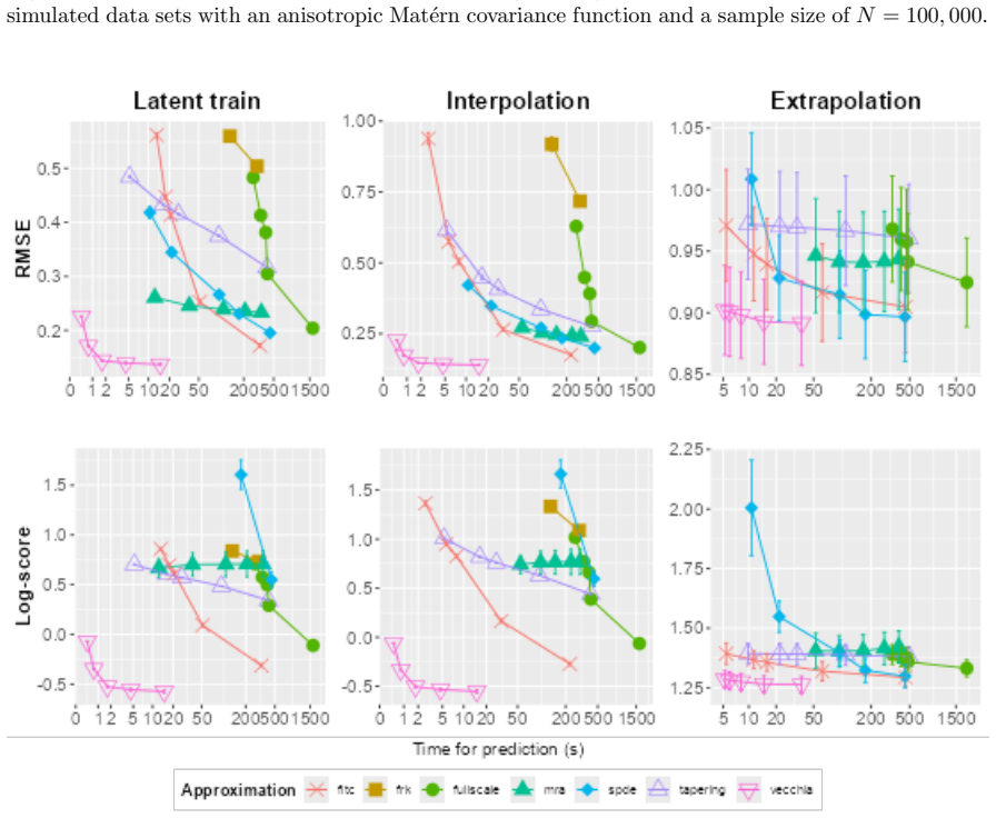
Gaussian processes (GPs) are flexible, probabilistic, nonparametric models widely used in fields such as spatial statistics and machine learning. A drawback of Gaussian processes is their computational cost, with $O(N^3)$ time and $O(N^2)$ memory complexity, which makes them prohibitive for large data sets. Numerous approximation techniques have been proposed to address this limitation. In this work, we systematically compare the accuracy of different Gaussian process approximations with respect to likelihood evaluation, parameter estimation, and prediction, explicitly accounting for the computational time required. We analyze the trade-off between accuracy and runtime on multiple simulated and large-scale real-world data sets and find that Vecchia approximations consistently provide the best accuracy-runtime trade-off across most settings considered.
Editorial analysis
A structured set of objections, weighed in public.
Referee Report
Summary. The manuscript conducts an empirical comparison of multiple scalable Gaussian process approximations (including Vecchia, inducing point, and others) for spatial data, evaluating accuracy in likelihood evaluation, parameter estimation, and prediction while accounting for runtime. It concludes that Vecchia approximations provide the best accuracy-runtime trade-off across most of the simulated and real-world datasets considered.
Significance. If the experimental comparisons are shown to be robust, this would offer practical guidance to spatial statisticians and machine learning practitioners facing large-N GP problems, where computational cost is a primary barrier. The work is a benchmarking study with no parameter-free derivations or machine-checked proofs, so its value rests entirely on the quality and representativeness of the empirical results.
major comments (2)
- [Abstract] Abstract: the headline claim that Vecchia approximations 'consistently provide the best accuracy-runtime trade-off across most settings considered' rests on the unverified assumptions that the chosen datasets span typical ranges of correlation lengths, observation densities, and non-stationarity, and that all implementations were comparably optimized (language, vectorization, convergence tolerances). No quantitative description of the data-generating processes or code-level controls is supplied, so the ranking cannot be assessed for robustness.
- [Methods] Methods/Experimental design (inferred from abstract): without explicit reporting of how runtime was measured (wall-clock on identical hardware, same hyper-parameter optimization protocol, etc.) or how accuracy metrics were normalized across methods, the accuracy-runtime trade-off curves cannot be interpreted as a fair comparison; this directly affects the central empirical ranking.
Simulated Author's Rebuttal
We thank the referee for their constructive comments on the robustness of our empirical study. We address each major comment below and have revised the manuscript to provide greater transparency on the experimental design and data-generating processes.
read point-by-point responses
-
Referee: [Abstract] Abstract: the headline claim that Vecchia approximations 'consistently provide the best accuracy-runtime trade-off across most settings considered' rests on the unverified assumptions that the chosen datasets span typical ranges of correlation lengths, observation densities, and non-stationarity, and that all implementations were comparably optimized (language, vectorization, convergence tolerances). No quantitative description of the data-generating processes or code-level controls is supplied, so the ranking cannot be assessed for robustness.
Authors: We agree that the abstract claim benefits from explicit support. The revised manuscript now includes a dedicated paragraph in Section 4.1 quantifying the simulated data-generating processes (correlation lengths ranging from 0.05 to 5 times the spatial domain diameter, observation densities from 10 to 500 points per unit area, and controlled non-stationarity via spatially varying length-scale functions). All methods were coded in R with equivalent vectorization and the same L-BFGS optimizer and convergence tolerances; these implementation controls are now summarized in Section 3.2 with pointers to the public repository. The abstract has been lightly edited to reference these details. revision: yes
-
Referee: [Methods] Methods/Experimental design (inferred from abstract): without explicit reporting of how runtime was measured (wall-clock on identical hardware, same hyper-parameter optimization protocol, etc.) or how accuracy metrics were normalized across methods, the accuracy-runtime trade-off curves cannot be interpreted as a fair comparison; this directly affects the central empirical ranking.
Authors: We have expanded the Methods section (now Section 3.3) to state that all runtimes are wall-clock measurements on identical hardware (Intel Xeon E5-2680 v4, 64 GB RAM) under the same hyper-parameter optimization protocol (L-BFGS with maximum 200 iterations and identical gradient tolerances). Accuracy metrics (negative log-likelihood, parameter RMSE, and predictive RMSE) were computed using the same definitions for every method without post-hoc normalization that would favor one approach. These additions directly address interpretability of the trade-off curves. revision: yes
Circularity Check
Empirical benchmarking study contains no derivations or load-bearing self-referential steps
full rationale
The paper is a systematic empirical comparison of GP approximations on simulated and real-world spatial datasets, evaluating accuracy-runtime trade-offs for likelihood, estimation, and prediction. No equations, parameter fits, or uniqueness theorems are presented as derivations; the central claim rests directly on observed experimental rankings across the tested settings. No self-citation chains, ansatzes, or renamings of known results appear in the load-bearing positions. This is the standard case of a self-contained benchmarking study whose validity depends on data representativeness and implementation fairness rather than any internal definitional reduction.
Axiom & Free-Parameter Ledger
Forward citations
Cited by 1 Pith paper
-
A new framework for non-stationary spatio-temporal data fusion of multi-fidelity models
A decomposed multi-fidelity covariance formulation allows Vecchia approximation on latent processes and GLS mean removal to deliver scalable, fully likelihood-based fusion of noisy low-fidelity and accurate high-fidel...
Reference graph
Works this paper leans on
-
[1]
18 Q. Pan, S. Abdulah, M. G. Genton, D. E. Keyes, H. Ltaief, and Y. Sun. GPU-Accelerated Vecchia Approximations of Gaussian Processes for Geospatial Data using Batched Matrix Computations. InISC High Performance 2024 Research Paper Proceedings (39th International Conference), pages 1–12. Prometeus GmbH,
work page 2024
-
[2]
F. D. Schneider, F. Morsdorf, B. Schmid, O. L. Petchey, A. Hueni, D. S. Schimel, and M. E. Schaepman. Data by Schneider et al. (2017) Mapping Functional Diversity from Remotely Sensed Morphological and Physiological Forest Traits. 3
work page 2017
-
[3]
ISSN 00359246. 19 Appendix A.1 Additional figures Figure 16: Average negative log-likelihood on simulated data sets with a practical range of 0.2 and a sample sizeN= 100,000. The true data-generating parameters are used on the left and “wrong” parameters obtained by doubling the true ones are used on the right. Figure 17: Bias and MSE of the estimates for...
work page 2000
-
[4]
0.43 36.3 1.27 11.3 13.6 6.99 Time (s) 3.37 15 23.6 49.3 19.3 16.1 Table 18: Average RMSE between means, RMSE between variances, KL divergence between exact and approximate predictions, standard errors and time needed for making predictions on the test “extrapolation” set on simulated data sets with an effective range of 0.2 and a sample size of N=10,000....
work page 1931
-
[5]
1.83e-04 4.17e-04 1.28e-03 6.7e-04 5.52e-03 5.45e-03 0.0178 KL 1214 4960 2035 4074 44168 2105 269 (SE
work page 2035
-
[6]
15.4 181 0.332 6.18 39.7 31.1 Time (s) 3.34 15.5 23.6 49.5 26.3 14.6 Table 30: Average RMSE between means, RMSE between variances, KL divergence between exact and approximate predictions, standard errors and time needed for making predictions on the test “extrapolation” set on simulated data sets with an effective range of 0.5 and a sample size of N=10,00...
work page 2065
-
[7]
1.17e-06 2.78e-05 6.45e-05 4.64e-05 1.06e-03 6.74e-05 1.57e-04 KL 38.4 2094 3878 3245 4566 969 26771 (SE
work page 2094
-
[8]
2.47e-05 1.83e-04 1.45e-04 1.94e-04 7.28e-03 3.3e-04 2.04e-04 KL 163 4421 8301 6057 8509 2062 70297 (SE
work page 2062
-
[9]
1.42e-06 1.33e-04 2.98e-04 1.77e-04 1.94e-04 2.72e-04 KL 5.89 1910 4988 2482 886 4526 (SE
work page 1910
-
[10]
0.0485 0.0364 0.0484 0.0457 0.0478 0.0598 Time (s) 46.5 475 451 1981 475 695 Table 50: Average RMSE and log-score on the test “extrapolation” set, standard errors and time needed for making predictions on the test “extrapolation” set on simulated data sets with an effective range of 0.2 and a sample size of N=100,000. 72 B.5 Simulated data withN= 100,000a...
work page 1981
-
[11]
0.0698 0.0527 0.0683 0.0621 0.0633 0.0847 Time (s) 46.4 510 453 1972 846 1207 Table 59: Average RMSE and log-score on the test “extrapolation” set, standard errors and time needed for making predictions on the test “extrapolation” set on simulated data sets with an effective range of 0.5 and a sample size of N=100,000. 82 B.6 Simulated data withN= 100,000...
work page 1972
-
[12]
1.24e-07 0.0826 4.84e-04 5.09e-06 1.13e-06 1.24e-06 Time (s) 20.7 250 61.3 133 1719 1954 4 Bias -5.92e-05 1.22 0.0254 5.99e-03 1.85e-03 3.31e-03 (SE
work page 1954
-
[13]
7.34e-04 1.84e-03 0.819 1.13e-03 9.83e-03 0.471 Time (s) 20.7 250 61.3 133 1719 1954 4 Bias -0.0131 -0.272 1.78 -0.0334 0.171 4.08 (SE
work page 1954
-
[14]
2.45e-06 6.08e-04 5.78e-03 6.62e-04 5.02e-06 4.57e-06 Time (s) 20.7 250 61.3 133 1719 1954 4 Bias 2.55e-04 -0.178 0.112 -0.141 1.68e-03 1.94e-03 (SE
work page 1954
-
[15]
0.0153 0.0156 0.0155 0.0158 0.0174 0.0178 Time (s) 46.4 463 452 1908 131 737 Table 68: Average RMSE and log-score on the test “extrapolation” set, standard errors and time needed for making predictions on the test “extrapolation” set on simulated data sets with an effective range of 0.05 and a sample size of N=100,000. 92 B.7 Simulated data withN= 100,000...
work page 1908
-
[16]
0.0177 0.0216 0.0199 0.0179 0.0341 0.0243 Time (s) 37.5 491 451 1942 386 448 Table 77: Average RMSE and log-score on the test “extrapolation” set, standard errors and time needed for making predictions on the test “extrapolation” set on simulated data sets with an anisotropic Mat´ ern covariance function and a sample size N=100,000. 100 B.8 Simulated data...
work page 1942
-
[17]
0.027 0.0357 0.0229 0.0282 0.0295 0.0342 Time (s) 46.5 491 452 1919 496 1186 Table 86: Average RMSE and log-score on the test “extrapolation” set, standard errors and time needed for making predictions on the test “extrapolation” set on simulated data sets with an effective range of 0.2, error variance of 0.1 and a sample size N=100,000. 110 B.9 Simulated...
work page 1919
-
[18]
2.67e-05 1921 834 0.0742 8.66e-04 8.65e-06 Time (s) 2.17 65.8 1.48 28.5 457 343 12.1 2 Bias 2.82e-03 173 0.483 0.102 0.0493 -0.0138 (SE
work page 1921
-
[19]
0.029 0.0322 0.0273 0.0281 0.029 0.0519 Time (s) 46.3 479 453 1898 97.2 597 Table 95: Average RMSE and log-score on the test “extrapolation” set, standard errors and time needed for making predictions on the test “extrapolation” set on simulated data sets with an effective range of 0.2, Mat´ ern smoothness of 0.5 and a sample size N=100,000. 120 B.10 Simu...
work page 2000
-
[20]
2.83e-05 0.0215 4.3e-04 2.37e-04 3.57e-05 3.83e-05 Time (s) 4.17 88.5 44 96.5 1973 113 3 Bias 2.66e-04 0.164 0.027 0.0179 0.0117 0.0117 (SE
work page 1973
-
[21]
0.022 5.39e-03 3.1 1.19 0.0943 0.787 Time (s) 4.17 88.5 44 96.5 1973 113 3 Bias 0.0332 -0.13 1.58 1.14 0.605 2.86 (SE
work page 1973
-
[22]
1.52e-06 2.78e-03 8.39e-06 1.71e-04 1.46e-06 1.34e-06 Time (s) 4.17 88.5 44 96.5 1973 113 3 Bias -4.74e-04 -0.24 -2.74e-03 -0.0331 -2.78e-04 -4.47e-04 (SE
work page 1973
-
[23]
0.0343 0.037 0.0362 0.0381 0.0328 0.037 Time (s) 46.6 480 452 1974 936 2315 Table 104: Average RMSE and log-score on the test “extrapolation” set, standard errors and time needed for making predictions on the test “extrapolation” set on simulated data sets with an effective range of 0.2, Mat´ ern smoothness of 2.5 and a sample size N=100,000. 130 B.11 Sim...
work page 1974
-
[24]
0.0337 0.037 0.0382 0.0371 0.0309 0.183 Time (s) 46.3 478 451 1944 98 599 Table 113: Average RMSE and log-score on the test “extrapolation” set, standard errors and time needed for making predictions on the test “extrapolation” set on simulated data sets with an effective range of 0.2, misspecified Mat´ ern smoothness and a sample size N=100,000. 140 B.12...
work page 1944
-
[25]
1.15e-05 0.315 9.98e-06 1.21e-04 4.18e-05 2.7e-05 Time (s) 135 4068 1986 2267 3690 6684 5 Bias -7.72e-04 1.74 -1.59e-03 8.01e-04 0.0137 6.08e-03 (SE
work page 1986
-
[26]
9.95e-03 0.0111 0.0218 0.373 0.0684 1.36 Time (s) 135 4068 1986 2267 3690 6684 5 Bias -0.0205 -0.51 -9.38e-04 0.172 0.534 3.51 (SE
work page 1986
-
[27]
1.76e-06 1.09e-03 5.51e-06 4.11e-05 1.8e-06 2.26e-06 Time (s) 135 4068 1986 2267 3690 6684 5 Bias 8.42e-04 -0.101 -6.51e-04 -7.94e-03 9.05e-04 1.65e-03 (SE
work page 1986
-
[28]
0.0485 0.0364 0.0484 0.0457 0.0478 0.0567 Time (s) 312 1710 2015 2294 477 1892 Table 145: Average RMSE and log-score on the test “extrapolation” set, standard errors and time needed for making predictions on the test “extrapolation” set on simulated data sets with an effective range of 0.2 and a sample size of N=100,000 in the single-core setting. 169 B.1...
work page 2015
discussion (0)
Sign in with ORCID, Apple, or X to comment. Anyone can read and Pith papers without signing in.