REVIEW 5 major objections 6 minor 19 references
ATSFFT: A Novel Sparse Fast Fourier Transform Enabled With Sparsity Detection
T0 review · 5 major / 6 minor · reviewed 2026-08-14 · deepseek-v4-flash
Pith's one-line read Adaptive tuning lets a two-dimensional sparse Fourier transform estimate its own sparsity k by counting local maxima in a hashed grid, then finish the transform without knowing k in advance.
desk verdict The sparsity-detection claim is supported by one example and the Eq. 8 hash is mis-specified; the paper is an extended experimental version of the authors' 2017 work, not a new algorithm. read the letter →
The pith
A machine-rendered reading of the paper's core claim, the machinery that carries it, and where it could break.
The reading
What carries the argument
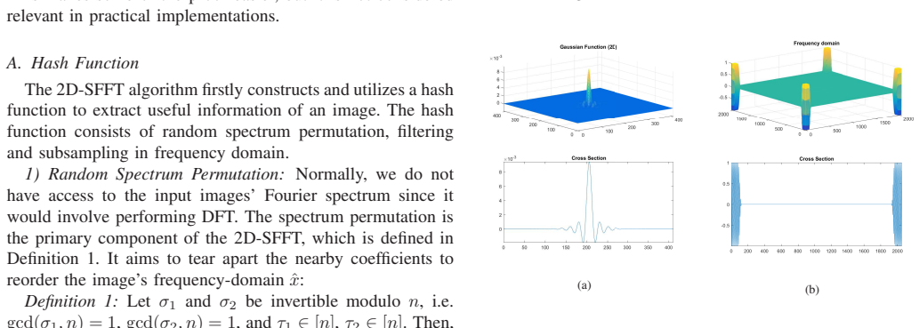
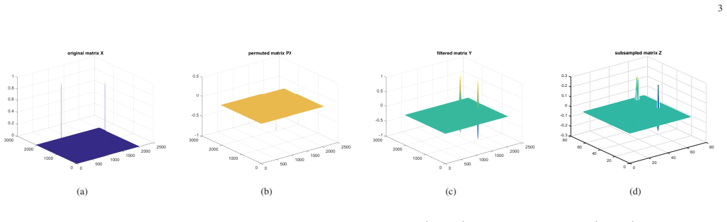
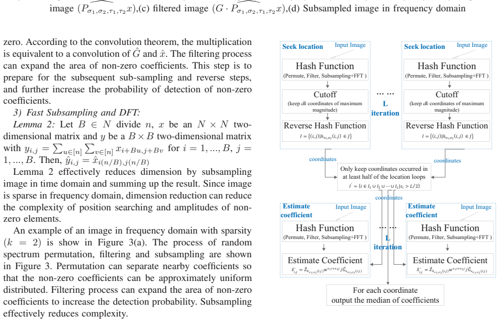
The load-bearing object is the two-dimensional hash function $h_{\sigma_1,\sigma_2}(i,j) = \mathrm{round}(\sigma_1 \sigma_2 i j B^2/N^2)$, assembled from random spectrum permutation, a two-dimensional flat Gaussian window filter, and fast subsampling with an FFT of size $B \times B$. This hash maps $N \times N$ frequency coordinates into $B \times B$ bins and is supposed to concentrate the image's nonzero coefficients into exactly $k$ local maxima, making sparsity observable. The adaptive controller built on that count, the update rules in Eq. (12), is what distinguishes ATSFFT from a standard sparse FFT: instead of taking $k$ as an input and fixing $B = \sqrt{Nk}$, it tunes $B$ by powers of two until successive sparsity estimates agree. The reverse-hash and median-based coefficient estimation stages then convert the stabilized bin information into explicit coordinates and amplitudes.
What would settle it
Take a synthetic $N \times N$ image with known sparsity $k$, choose the nonzero frequency coordinates randomly, run the hash function for many trials, and count local maxima in the resulting $B \times B$ matrix; if any trial yields a count different from $k$, the central equality asserted in Section III.A is false. A targeted version places two nonzero coefficients so that, after permutation and filtering, their hash bins are adjacent and their filter spreads merge into a single local maximum.
Extended reading notes
Core claim
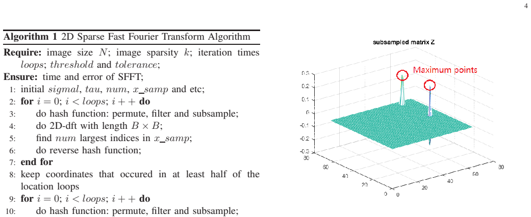
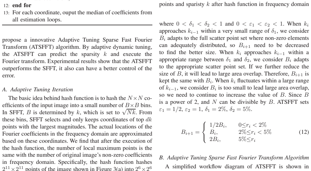
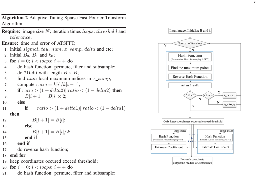
The paper's central discovery is that unknown sparsity can be probed rather than assumed: after the hash function, the number of local maxima in the hashed $B \times B$ magnitude matrix is asserted to be the same as the image's sparsity $k$. Starting from an initial small $B_0$, the algorithm counts local maxima to obtain $k_1$, defines the change ratio $r_i = |1 - k_i/k_{i-1}|$, and updates the bin size by $B_{i+1}=B_i/2$ when $r_i < 2\%$, $B_{i+1}=B_i$ when $2\% \le r_i < 5\%$, and $B_{i+1}=2B_i$ when $r_i \ge 5\%$. Once $B$ and $k$ stabilize, candidate coordinates are collected by reverse hashing from locations that appear in at least half of the seek loops, and each coefficient is taken as the median of repeated estimation rounds. The paper reports that this self-tuning procedure runs faster than both the original sparse FFT and FFTW, with smaller average L1 error on the tested sparse images.
Load-bearing premise
The whole sparsity-detection mechanism rests on the assertion that after hashing, the number of local maxima in the $B \times B$ matrix equals the true sparsity $k$; if that count is off, the adaptive loop estimates the wrong $k$ and the update rules for $B$ have no justification.
Editorial extensions
If this is right
- Users no longer need to know or guess the sparsity $k$ before running the transform, so sparse FFT can be applied where signals are only known to be sparse in the frequency domain.
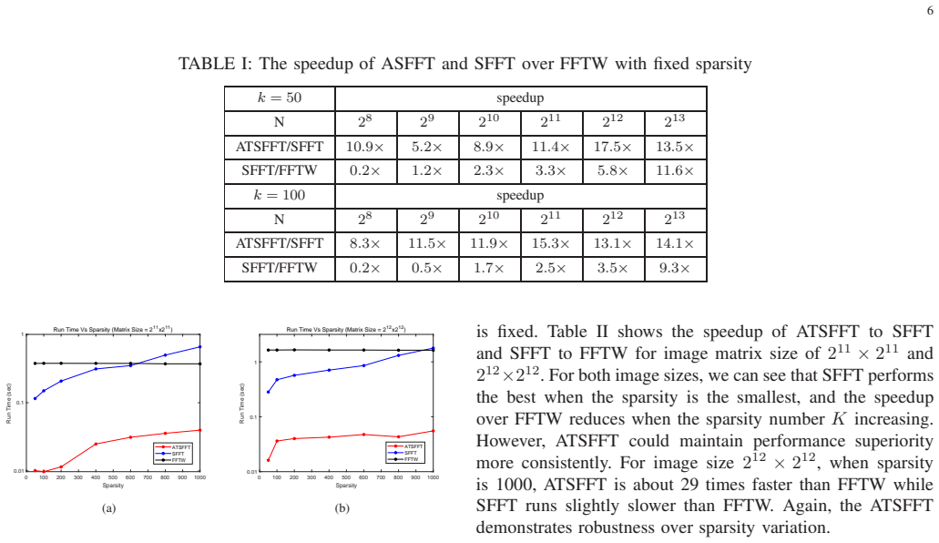
- Because $B$ adapts to the signal rather than being fixed by an assumed $k$, runtime stays low as sparsity varies; reported runtimes for $N=2^{11}$ and $N=2^{12}$ remain under 0.1 seconds across $k$ from 50 to 1000.
- The method extends the range where sparse FFT beats FFTW: at $N=2^{12}$ and $k=1000$, the earlier sparse FFT is slower than FFTW while ATSFFT remains faster.
- Reported error decreases as image size grows for fixed sparsity, meaning the method becomes more accurate precisely in the large-image regime where its speed advantage is largest.
Reading between the lines
- If local-maximum counting is only reliable when the random permutation spreads nonzero coefficients far apart, then the correctness of the sparsity probe is probabilistic; a reader should expect a formal bound on the chance that two nonzeros merge into one peak, but the paper does not supply one.
- The hash in Eq. (8) maps a 2D coordinate to a single rounded integer rather than a pair of bin indices; a testable extension would compare this scheme with separable row and column hashing to see which gives more stable local-maximum counts.
- The update thresholds 2% and 5% are fixed constants; they could be tuned per signal class or made to depend on $N$ and $B$, and the paper leaves that margin unexamined.
- Because the equality between local maxima and $k$ is demonstrated with a single example, a natural next step is to measure the failure rate of that equality over random coefficient placements and window parameters.
Signed reviews
Editorial analysis
A structured set of objections, weighed in public.
Referee Report
Summary. The paper proposes ATSFFT, an adaptive two-dimensional sparse fast Fourier transform whose main novelty is automatic detection of the unknown sparsity k. The algorithm is built on a hash-based binning procedure followed by adaptive tuning of the bin size B; the number of local maxima in the hashed B×B matrix is claimed to equal k. The paper reports experiments on synthetic k-sparse images comparing runtime, speedup, and error against SFFT and FFTW, claiming that ATSFFT controls error better than SFFT and achieves an order-of-magnitude speedup over FFTW. The central mechanism, the sparsity probe, is asserted rather than proved, and several technical details of the hash and tuning loop are not adequately specified.
Significance. If the sparsity-detection identity were proven and the algorithm fully specified, an adaptive sparse FFT for the unknown-sparsity setting would be a useful practical contribution. The paper does not, however, deliver such a proof or specification. The main claim rests on a single k=2 example, the hash function as written does not map to a two-dimensional bin grid, the tuning thresholds are ad hoc, and the paper's own error tables contradict the claimed error-control advantage. The manuscript's positive aspects are the clear identification of a real limitation in SFFT (the need to know k in advance) and a substantial set of runtime comparisons; however, without a valid sparsity-detection mechanism the central contribution is not established.
major comments (5)
- [Section III.A, Eq. (8)] The central sparsity-detection claim—that after hashing, the number of local maxima in the B×B matrix equals the number of non-zero Fourier coefficients—is asserted with a single k=2 example and no proof. This identity is the load-bearing step of the adaptive tuning loop, and it cannot be taken as self-evident: collisions, filter leakage, and the choice of B can change the local-maximum count. Furthermore, h(i,j)=round(σ1σ2ijB^2/N^2) maps a coordinate (i,j) to a single integer in [B^2], not to a pair of bin indices in [B]×[B]; the paper does not state how this integer is converted to a 2D bin, nor does it define the reverse hash function needed to map candidate bins back to frequency coordinates. The algorithm is therefore not fully specified at its core.
- [Section III.A, Eqs. (10)-(12)] The update rules for B and the thresholds δ1=2%, δ2=5%, ε1=1/2, ε2=1 are introduced without derivation, convergence analysis, or sensitivity study. The textual rationale (e.g., that a small value of r_i means B is 'adapted to the full scatter point set') is not connected to a formal model of how the local-maximum count depends on B, and no experiment isolates the tuning loop's behavior. I note that I do not find a contradiction between Algorithm 2 and Eq. (12); in terms of r_i, small r_i triggers B/2 and large r_i triggers 2B in both places. The problem is that neither the definition of r_i nor the threshold choices is justified, which is a major gap for an algorithm whose entire contribution is automatic sparsity detection.
- [Section IV, Table IV] The conclusion that 'ATSFFT can control the error better than SFFT' is contradicted by the reported data. For N=2^12 with k=100, ATSFFT has error 3.69×10^-10 versus 2.38×10^-10 for SFFT; for k=400, 2.54×10^-5 versus 2.64×10^-6; for k=600, 4.73×10^-5 versus 1.27×10^-5. These entries show SFFT with strictly lower error, so the abstract and Section IV-C overstate the error-control advantage.
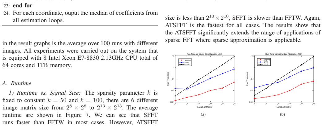
- [Section IV-B, Table I] The claimed order-of-magnitude speedup over FFTW is not uniform. At N=2^8, SFFT/FFTW is 0.2 and ATSFFT/SFFT is 10.9, giving ATSFFT only about 2.2× over FFTW. The paper provides no error bars, no statistical significance tests, and no complexity bound for the adaptive loop, so the performance claims are not established across the reported parameter range.
- [Section IV] All experiments use exactly k-sparse synthetic images with random support and unit magnitudes. This is the most favorable regime for the unproven local-maximum-count identity, and it does not test the method's stated motivation of handling real images with approximate frequency sparsity. No experiment reports the accuracy of the sparsity estimate k_i itself, so there is no direct evidence that the adaptive probe detects k correctly.
minor comments (6)
- [Section V] The conclusion refers to 'the paper in Section II-B', which is incorrect; it should refer to the conclusion section.
- [Throughout] There are numerous typographical errors ('tow-dimensional', 'practival', 'equiped', 'sigmal', 'sparisty', 'Morever') and inconsistent notation ('A TSFFT' vs 'ATSFFT') that should be corrected.
- [Section II.A] The text says 'By applying convolution of (8) and (9)', but the filter and window are defined in Eqs. (6) and (7); Eq. (8) is the hash function introduced later.
- [Figures 4 and 5] The caption and text disagree about the figure number, the caption says '2D-SFT' instead of '2D-SFFT', and Figure 5's caption appears without the corresponding plot in the text.
- [Introduction] The citation placeholder 'radio astronomy[reference]' should be completed.
- [Algorithm 2] The variable names (sigmal, x samp, ratio) are undefined or inconsistent with Section III.A's r_i, and the role of initial k0 in the first iteration is not explained.
Circularity Check
No significant circularity: the ATSFFT sparsity-detection claim is unsupported but not equivalent to its inputs by construction.
full rationale
The paper's derivation chain is self-contained: the permutation, filtering, and subsampling steps are stated as Lemmas 1 and 2 and proved in-text, and the ATSFFT tuning loop is described with its own update rule in Eq. (12). The central load-bearing assertion, "after the execution of the hash function, the number of local maximum points is the same with the number of original image's non-zero coefficients in frequency domain" (Section III.A), is supported only by a k=2 example and is not proved; however, it is an empirical heuristic about the relation between a computed statistic and the true sparsity, not a quantity that is defined in terms of the target result. The tunable thresholds (delta1=2%, delta2=5%, eps1=1/2, eps2=1) are stated as fixed constants rather than fitted parameters, and no fitted input is renamed as a prediction. The self-citations [17] and [18] describe the authors' prior 2D-SFFT and ATSFFT work, but the present paper does not rely on those citations for the key tuning claim; it reproduces the algorithmic description in the text. No uniqueness theorem is imported from the authors' prior work, and no known result is merely renamed. The inconsistency between the hash function in Eq. (8) and the 2D bin structure, and the lack of proof for the local-max-to-k identity, are correctness and rigor concerns, not circularity. Therefore the appropriate circularity score is 0.
Assumptions & free parameters
free parameters (5)
- delta1 threshold =
2%
- delta2 threshold =
5%
- B update multiplier epsilon1 =
1/2
- B update multiplier epsilon2 =
1
- initial B0 and k0 =
not specified
assumptions (4)
- domain assumption Signals of interest are sparse in the frequency domain (images have few non-zero Fourier coefficients).
- domain assumption The hash function h(i,j) maps non-zero frequencies to distinct bins with high probability.
- ad hoc to paper The number of local maxima in the B x B hashed matrix equals the true sparsity k.
- standard math Standard DFT properties and the convolution theorem hold as used in Lemmas 1 and 2.
Cite this review
Pith. "Pith review of ATSFFT: A Novel Sparse Fast Fourier Transform Enabled With Sparsity Detection." pith.science (2026). https://pith.science/paper/KSJGNSNH
@misc{pith2026190802461,
  author       = {Pith},
  title        = {Pith review of: ATSFFT: A Novel Sparse Fast Fourier Transform Enabled With Sparsity Detection},
  year         = {2026},
  howpublished = {\url{https://pith.science/paper/KSJGNSNH}},
  note         = {Machine review of arXiv:1908.02461}
}
abstract
The Fast Fourier Transform(FFT) is a classic signal processing algorithm that is utilized in a wide range of applications. For image processing, FFT computes on every pixel's value of an image, regardless of their properties in frequency domain. The Sparse Fast Fourier Transform (SFFT) is an innovative algorithm for discrete Fourier transforms on signals that possess characteristics of the sparsity in frequency domain. A reference implementation of the algorithm has been proven to be efficient than modern FFT library in cases of sufficient sparsity. However, the SFFT implementation has a critical drawback that it only works reliably for very specific input parameters, especially signal sparsity $k$, which hinders the extensive application of SFFT. In this paper, we propose an Adaptive Tuning Sparse Fast Fourier Transform (ATSFFT), which is a novel sparse fast fourier transform enabled with sparsity detection. In the case of unknown sparsity $k$, ATSFFT is capable of probing the sparsity $k$ via adaptive dynamic tuning and completing the sparse Fourier transform. Experimental results show that ATSFFT outperforms SFFT while it is able to control the computation error better than SFFT. Furthermore, ATSFFT achieves an order of magnitude of performance improvement than the state-of-the-art FFT library, FFTW.
Figures

Figures from the paper (6 more)
Reference graph
Works this paper leans on
-
[1]
C.F.Beckmann and S.M.Smith, ”Probabilistic independe nt component analysis for functional magnetic resonance imaging,” IEEE Transactions on Medical Imaging, vol.23,no.2,pp.137-152,2004
work page 2004
-
[2]
Shota Taki, Fumihiko Sakaue, and Jun Sato, ”High resolut ion light field photography from split ray imaging and coded aperture,” in V ISAPP 2014-Proceedings of the 9th International Conference on Co mputer Vision Theory and Applications, V olume 2, Lisbon, Portugal, 5-8 January, 2014, pp.605-612
work page 2014
- [3]
-
[4]
Geos cience and Remote Sensing, vol
Jon Atli Benediktsson, Martino Pesaresi, and Kolbeinn A mason, ”Classs- fication and feature extraction for remote sensing images fr om urban areas based on morphological transformations,” IEEE Trans. Geos cience and Remote Sensing, vol. 41, no.9,pp.1940-1949, 2003
work page 1940
-
[5]
S. Grace Chang, Bin Y u, and Martin V etterli, ”Adaptive wa velet thresh- olding for image denoising and compression,” IEEE Trans. Im age Pro- cessing, vol.0, no.9,pp.1532-1546, 2000
work page 2000
- [6]
-
[7]
B. S. Reddy and B. N. Chatterji, ”An FFT-based technique f or translation, rotation, and scale-invariant image registration,” in IEE E Transactions on Image Processing, vol. 5, no. 8, pp. 1266-1271, Aug 1996
work page 1996
- [8]
Show all 19 references
-
[9]
S. Ma, X. Zhang, J. Zhang, C. Jia, S. Wang and W. Gao, ”Nonlo cal In- Loop Filter: The Way Toward Next-Generation Video Coding?, ” in IEEE MultiMedia, vol. 23, no. 2, pp. 16-26, Apr.-June 2016
2016
-
[10]
Zhang, W
X. Zhang, W. Lin, R. Xiong, X. Liu, S. Ma and W. Gao, ”Low-R ank Decomposition-Based Restoration of Compressed Images via Adaptive Noise Estimation,” in IEEE Transactions on Image Processin g, vol. 25, no. 9, pp. 4158-4171, Sept. 2016
2016
-
[11]
Zhang, W
X. Zhang, W. Lin, S. Wang and S. Ma, ”Nonlocal Adaptive In -Loop Filter via Content-Dependent Soft-Thresholding for HEVC, ” 2015 IEEE International Symposium on Multimedia (ISM), Miami, FL, 20 15, pp. 465-470
2015
-
[12]
Zhang, W
X. Zhang, W. Lin, J. Liu and S. Ma, ”Compression noise est imation and reduction via patch clustering,” 2015 Asia-Pacific Signal a nd Information Processing Association Annual Summit and Conference (APSI PA), Hong Kong, 2015, pp. 715-718
2015
-
[13]
Zhang, R
X. Zhang, R. Xiong, X. Fan, S. Ma and W. Gao, ”Compression Artifact Reduction by Overlapped-Block Transform Coefficient Estim ation With Block Similarity,” in IEEE Transactions on Image Processin g, vol. 22, no. 12, pp. 4613-4626, Dec. 2013
2013
-
[14]
S. Shi, R. Xiong, S. Ma, X. Fan and W. Gao, ”Image compress ive sensing using overlapped block projection and reconstruct ion,” 2015 IEEE International Symposium on Circuits and Systems (ISCAS), L isbon, 2015, pp. 1670-1673
2015
-
[15]
1183–1194
Haitham Hassanieh, Piotr Indyk, Dina Katabi and Eric Pr ice,”Simple and practical algorithm for sparse Fourier transform,” Pro ceedings of the Twenty-Third Annual ACM-SIAM Symposium on Discrete Algori thms, 2012, Japan, pp. 1183–1194
2012
-
[16]
563–5 78
Haitham Hassanieh, Piotr Indyk, Dina Katabi and Eric Pr ice,”Nearly optimal sparse fourier transform,” Proceedings of the 44th Symposium on Theory of Computing Conference, 2012, New Y ork, pp. 563–5 78
2012
-
[17]
S. Shi, R. Y ang and H. Y ou, ”A new two-dimensional Fourie r transform algorithm based on image sparsity,” 2017 IEEE Internationa l Conference on Acoustics, Speech and Signal Processing (ICASSP), New Or leans, LA, 2017, pp. 1373-1377
2017
-
[18]
S. Shi, R. Y ang, X. Zhang, H. Y ou, D. Fan, ”An Adaptive Tun ing Sparse Fast Fourier Transform”, Advances in Multimedia Informati on Processing (PCM) 2017. Lecture Notes in Computer Science, vol 10736
2017
-
[19]
Frigo and S
M. Frigo and S. G. Johnson, ”FFTW: an adaptive software a rchitecture for the FFT,” Acoustics, Speech and Signal Processing, 1998 . Proceedings of the 1998 IEEE International Conference on, Seattle, W A, 1 998, pp. 1381-1384
1998
Reviewed August 14, 2026 · model on record in the stance chip above.
Discussion (0). Continue with ORCID to comment.