REVIEW 4 major objections 6 minor 36 references
Turbulent Injection assisted by Diffusion Models for Scale Resolving Simulations
T0 review · 4 major / 6 minor · reviewed 2026-08-06 · deepseek-v4-flash
Pith's one-line read A diffusion model conditioned on one Reynolds number can generate realistic turbulent inlet fields for LES/DNS, replacing stored precursor libraries.
desk verdict A promising ML-CFD proof-of-concept whose storage-free inflow generation works reasonably well, but the abstract overstates autocorrelation accuracy and the scalar Re_Lint conditioning does not actually control L_int. read the letter →
The pith
A machine-rendered reading of the paper's core claim, the machinery that carries it, and where it could break.
The reading
What carries the argument
The carrying mechanism is a classifier-free guided diffusion model: a UNet score network trained with the variance-preserving SDE objective to denoise $3\times64^3$ velocity boxes, conditioned on the scalar Reynolds number $Re_{L_{\mathrm{int}}} = \sqrt{2/3}\,k\,L_{\mathrm{int}}/\nu$. This single number is the interface between the user-specified turbulence state and the generated field — it is what lets the model interpolate across TKE/scale combinations without retraining. Temporal continuity between successive generated boxes, required for an inlet condition, is imposed by Moment Matching Posterior Sampling, which treats the last $m=16$ slices of the previous box as a noisy measurement co
What would settle it
Generate two DHIT boxes with the same $Re_{L_{\mathrm{int}}}$ but different pairs $(k, L_{\mathrm{int}})$ — for example, double $k$ and halve $L_{\mathrm{int}}$ so the product is unchanged — and condition the model at that Reynolds number. If the model produces the same energy spectrum and integral length scale for both, the conditioning is degenerate and the central premise fails.
Extended reading notes
Core claim
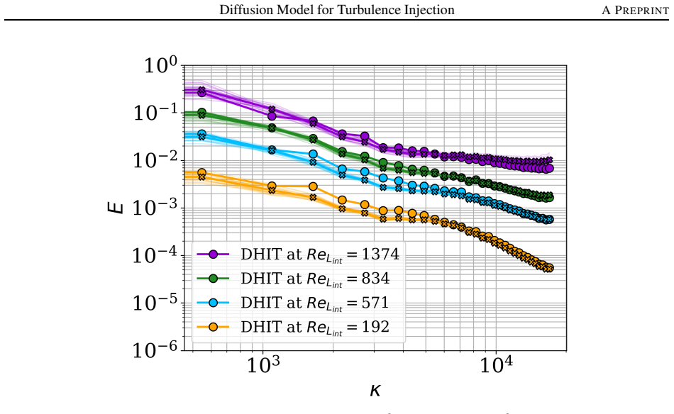
A classifier-free guided diffusion model trained on 214 DHIT boxes spanning $Re_{L_{\mathrm{int}}} \in [196.58, 1302.16]$ can generate new $64^3$ instantaneous velocity boxes whose a priori statistics (energy spectrum, vorticity distribution, Reynolds-stress anisotropy) closely match ground truth, and after injecting them at the inlet of a free-domain LES the turbulence develops as fast as with the original precursor method — in less than one box length for the energy spectrum at 23.3% turbulence intensity. The conditioning variable $Re_{L_{\mathrm{int}}}$ embeds both the turbulent kinetic energy level and the integral length scale, so a single model covers many target states and interpolate
Load-bearing premise
The load-bearing premise is that a single Reynolds number $Re_{L_{\mathrm{int}}}$ contains enough information to fix the turbulence statistics the model must generate; if two flows with different turbulent kinetic energies and integral length scales share the same Reynolds number, the conditioned samples cannot distinguish them.
Editorial extensions
If this is right
- Within the trained Reynolds-number range, the user can query any target TKE/length-scale state without running a new DHIT; 24 boxes are generated in about three minutes on the tested GPU setup.
- The inlet library no longer needs to be stored or read from disk: the model itself is the library, and successive boxes can be generated on demand.
- The development distance of the generated turbulence is not increased relative to the precursor method (1–2 box lengths, depending on turbulence intensity), so no extra fetch length must be added to the computational domain.
- The stochasticity of the diffusion model decorrelates successive inlet boxes: MMPS keeps the time correlation below 10%, unlike simply re-injecting one frozen DHIT box.
- The same model can be reused in the trial-and-error loop that matches an inlet condition to measurements at a target station, because regenerating at a new conditioning value costs seconds instead of a full precursor rerun.
Reading between the lines
- Not tested here: because conditioning is a single scalar, any two physical states with the same $Re_{L_{\mathrm{int}}}$ but different $(k, L_{\mathrm{int}})$ are indistinguishable to the model; conditioning separately on $k$ and $L_{\mathrm{int}}$ would directly test whether this embedding is lossy.
- The observed asymmetry — extrapolating to lower $Re_{L_{\mathrm{int}}}$ works well, extrapolating to higher does not — suggests a learned hierarchy in which lower-Reynolds fields are filtered versions of higher-Reynolds ones. A testable consequence is that a model trained on a longer decay sequence could generate new states by denoising downward rather than by inventing small scales.
- The MMPS inlet anisotropy (dominant $u'u'$ component) indicates that conditioning on $y$–$z$ slices constrains the streamwise velocity differently from the cross-stream components; adding a divergence-free projection during sampling, which the paper lists as a perspective, would be a direct test.
- Because the training set is built from periodic boxes with translation augmentation, the current proof is tied to homogeneous freestream turbulence; extending to boundary layers or wakes would require a non-periodic architecture and a different training representation.
Editorial analysis
A structured set of objections, weighed in public.
Referee Report
Summary. The paper proposes a classifier-free diffusion model trained on 214 three-dimensional snapshots of Decaying Homogeneous Isotropic Turbulence to generate instantaneous turbulent velocity boxes for use as inflow boundary conditions in LES/DNS. The model is conditioned on a scalar Reynolds number Re_Lint = sqrt(2/3 k)L_int/nu. Generated boxes are assessed a priori via energy spectra, two-point autocorrelations, barycentric anisotropy triangles, and vorticity PDFs, and a posteriori by injecting them into a free domain with two concatenation methods (blending and moment matching posterior sampling). The authors compare against a library-based precursor method and report similar development distances, lower storage, and faster turnaround for finding target TKE levels.
Significance. The manuscript addresses a real bottleneck in scale-resolving simulations: the high memory and setup cost of precursor-based turbulence inflow. It demonstrates that a diffusion model can generate 3D turbulent boxes with reasonable energy spectra and TKE at multiple Reynolds numbers, and that injected samples develop qualitatively as quickly as the precursor method. The computational cost comparison (Table 2, Fig. 21) and the use of MMPS for temporal continuity are useful contributions. However, the central claim about accurate reproduction of two-point statistics is not supported by the reported results, and the conditioning on a single scalar is not validated for length-scale control. With revisions, the method remains a promising proof-of-concept.
major comments (4)
- [Section 4.1 / Fig. 10 / Abstract] The abstract claims samples 'accurately reproduce turbulence statistics, such as the energy spectrum and the two-point autocorrelation functions.' The paper's own a priori results contradict this: §4.1 states there is 'an underestimation of f(r) and an overestimation of g(r)' and that 'The model seems to have difficulty distinguishing between the integral length scales and predicts the same correlations at each ReLint.' A posteriori, §4.2.1 reports L_int overestimated by about 14%; §4.2.2 reports about 20% relative error at x/L=4. Please quantify the errors on f(r), g(r), and L_int and revise the abstract and conclusions accordingly. This is not a presentation issue; it is the paper's headline result.
- [Section 4, Eq. (11)] The conditioning strategy assumes a single scalar Re_Lint = sqrt(2/3 k) L_int / nu uniquely determines the target statistics. The paper does not show identifiability: in the 214 training boxes, is L_int a deterministic function of Re_Lint? If two different (k, L_int) states share a Re_Lint value, or if the model cannot vary L_int at fixed Re_Lint, then a user specifying Re_Lint cannot target a desired vortex size. The failure to reproduce L_int (Figs. 10, 14, 18) is consistent with this identifiability problem. Please plot L_int vs Re_Lint for the training data and consider conditioning on TKE and L_int separately (e.g., two-channel conditioning) or justify why Re_Lint is sufficient.
- [Section 4.1, Eq. (12) and §3.2] The hyperparameters lambda*, tau*, gamma* and the MMPS parameters m, Sigma_y are selected by minimizing a loss (Eq. 12) that includes the same statistics (k, E(kappa), f/g, barycentric coordinate) used later for validation. Consequently, the reported a priori agreement is not independent evidence of generalization. Please perform a nested validation (e.g., a separate hyperparameter-selection split) or report sensitivity of the metrics to lambda, tau, gamma, m, Sigma_y. Note that the h_{f,g} term is weighted by 100, so the persistent failure of correlation functions is especially telling.
- [Sections 4.2.1-4.2.2 / Section 5] The a posteriori comparison rests on only two test conditions and on single trajectories without error bars or statistical significance over the 24 generated boxes. The statement 'The development distance of the two methods is approximately the same' (Section 5) is qualitative. Please define the development length quantitatively (e.g., distance to reach within a specified tolerance of the target TKE and spectrum) and report uncertainties. This is the main practical advantage claimed for the method.
minor comments (6)
- [Figure 9 caption] The caption contains a leftover internal note: 'Discuss more the limitation of a pure data-driven model...' Remove it before submission.
- [Eq. (5)] The definition of R_ij appears with a comma inside the ensemble average; it should be R_ij(r,t) = <u_i(x+r,t) u_j(x,t)>.
- [Section 2.3.1 / Table 1] The text counts 214 boxes and then says 62 boxes and 17 boxes are used for training and validation; the relationship to Table 1's training size 136,102 (after translations) should be stated clearly.
- [Figure 15 / Figure 20 captions] Both captions say 'three streamwise locations,' but the figures show eight panels. Correct the captions to match the displayed x/L values.
- [Table 2] The symbols ✓, ≈, and ✗ need a legend; the Storage row formatting (32MB GPUs, 72MB CPUs, 3MB CPUs) is confusing and should be clarified.
- [Section 2.3.2 / Section 6] 'descent synthetic turbulence' should be 'decent.' The conclusion should be toned down to reflect the L_int limitation rather than stating 'good agreement' without qualification.
Circularity Check
Partial circularity: sampling hyperparameters are tuned on the same statistics later reported as validation; the core generation is otherwise self-contained.
-
fitted input called prediction
[Section 3.2 (MMPS parameters) and Section 4.1, Eq. 12 (grid search for lambda, tau, gamma)]
"In Section 4, m and Σy are set to 16 and 10−4, respectively. These values are obtained by grid search and are those that best preserve the statistics of interest defined in Section 2. ... The optimal λ ∗, τ ∗, and γ ∗ are those how minimize the following loss, L (λ , τ, γ) = αkhk + αEκ hEκ + α f ,gh f ,g + α△h△, (12) where ... hk = |ˆk − k|/k, h△ = ∑ i 1(ξi,ηi) /∈△, hEκ = ... h f ,g = ..."
The sampling hyperparameters of the diffusion model (λ, τ, γ) and the continuation parameters of MMPS (m, Σy) are explicitly chosen by minimizing a loss built from the very statistics used for validation: TKE level, energy spectrum, autocorrelation functions, and barycentric realizability. The reported 'accurate reproduction' of these statistics is therefore a calibrated optimum of the evaluation metrics, not an independent prediction. This is partial rather than total circularity because the diffusion model must still generate the 3D velocity fields and the a posteriori injection comparisons provide a separate physical benchmark, but the headline statistical agreement is in part manufactured by the selection procedure.
full rationale
Most of the derivation is self-contained: the diffusion model is trained on DHIT snapshots and its output is tested against the precursor method in an actual free-domain injection. The cited prior work by co-authors (Rozet & Louppe; Rasquin et al.) supplies open-source sampling code and the baseline precursor method, not an unverified uniqueness theorem or a load-bearing self-citation. The conditioning on the scalar Re_Lint is an identifiability choice rather than a circular definition; indeed, the reported 14–20% errors in L_int show that the conditioning does not force the integral length scale, so the model's imperfect length-scale reproduction is a genuine empirical finding. The main circularity concern is the hyperparameter selection in Section 4.1 and Section 3.2: λ, τ, γ, m, and Σy are tuned to minimize errors on the same TKE, spectrum, correlation, and barycentric statistics that are later presented as validation. This makes the agreement on those metrics a calibrated optimum rather than an independent confirmation. It does not completely collapse the central claim because the generative model must still produce realistic 3D fields and the a posteriori development-length comparison is an independent physical test. The unedited note in the Figure 9 caption ('Discuss more the limitation of a pure data-driven model...') further acknowledges unresolved limitations, which supports a moderate rather than high circularity score.
Assumptions & free parameters
free parameters (6)
- lambda (Langevin corrections) =
4
- tau (reverse SDE step) =
0.1
- gamma (guidance scale) =
2
- m (MMPS slices) =
16
- Sigma_y (MMPS measurement variance) =
1e-4
- Loss weights alpha_k, alpha_E, alpha_fg, alpha_delta =
1, 1, 100, 1/ns
assumptions (5)
- domain assumption Taylor frozen turbulence hypothesis and spatial homogeneity hold at the inlet, so a frozen precursor box can be swept at the mean inlet velocity.
- domain assumption Decaying Homogeneous Isotropic Turbulence is a canonical representation of experimental freestream turbulence in front of blades and grids.
- ad hoc to paper The Reynolds number Re_Lint = sqrt(2/3 k) L_int / nu uniquely determines the turbulent state the model should generate.
- domain assumption Small scales below the DHIT resolution are restored naturally by the flow solver after injection.
- standard math The MMPS posterior sampling is a valid way to impose continuity between consecutive generated boxes.
Cite this review
Pith. "Pith review of Turbulent Injection assisted by Diffusion Models for Scale Resolving Simulations." pith.science (2026). https://pith.science/paper/KV7B6UT3
@misc{pith2026250804318,
  author       = {Pith},
  title        = {Pith review of: Turbulent Injection assisted by Diffusion Models for Scale Resolving Simulations},
  year         = {2026},
  howpublished = {\url{https://pith.science/paper/KV7B6UT3}},
  note         = {Machine review of arXiv:2508.04318}
}
read the original abstract
The present research proposes a new memory-efficient method using diffusion models to inject turbulent inflow conditions into Large Eddy Simulation (LES) and Direct Numerical Simulation (DNS) for various flow problems. A guided diffusion model was trained on Decaying Homogeneous Isotropic Turbulence (DHIT) samples, characterized by different turbulent kinetic energy levels and integral length scales. Samples generated by the diffusion model accurately reproduce turbulence statistics, such as the energy spectrum and the two-point autocorrelation functions, while preserving the ability to generate instantaneous three-dimensional velocity fields with detailed fluctuations. Physical representativeness is also evaluated by injecting the \textit{synthetic} samples into a free domain (i.e., without any wall boundary) through an inlet boundary condition. The method demonstrates promising results regarding energy spectrum, spatial correlation, turbulent kinetic energy level, and integral length scales without increasing the development distance as compared to a library-based method. The following article has been submitted to/accepted by Physics of Fluid (AIP Publishing LLC). After publication, it will be available https://doi.org/10.1063/5.0278541.
Figures


Figures from the paper (16 more)




Reference graph
Works this paper leans on
-
[12]
doi: 10.1063/5.0106664. Y . Dreze, M. Hao, and L. di Mare. Divergence-free turbulent i nflow data from realistic covariabce tensor. Physics of Fluids, 35:025120,
-
[15]
doi: 10.1016/j. ijheatfluidflow.2006.02.006. M. Pamiès, P .-E. Weiss, E. Garnier, S. Deck, and P . Sagaut. Ge neration of synthetic turbulent inflow data for large eddy simulation of spatially evolving wall-bounded flows. Physics of Fluids , 21(4):045103,
doi:10.1016/j 2006
-
[17]
doi: 10.1016/j.compfluid.2018.03.069 . D. Muñoz-Esparza, B. Kosovi ´c, J. van Beeck, and J. Mirocha. Erratum: “a stochastic pertu rbation method to generate inflow turbulence in large-eddy simulation models: Applica tion to neutrally stratified atmospheric boundary layers". Physics of Fluids , 27(3):039901,
doi:10.1016/j.comp 2018
-
[18]
doi: 10.1063/1.4915140. R. DeLeon, C. Umphrey, and I. Senocak. Turbulent inflow gener ation through buoyancy perturbations with colored noise. AIAA Journal, 57(2),
-
[19]
Anthony Keating and Ugo Piomelli
doi: 10.2514/1.J057245. Anthony Keating and Ugo Piomelli. A dynamic stochastic forc ing method as a wall-layer model for large-eddy simulation. Journal of Turbulence, 7:N12,
-
[20]
doi: 10.1080/1468524061233 1392460
ISSN 1468-5248. doi: 10.1080/1468524061233 1392460. M. Rasquin, T. Toulorge, M. Bechlars, and K. Hillewaert. DIR ECT NUMERICAL SIMULA TIONS OF AIR- FOIL CASCADES FOR THE IMPROVEMENT OF TURBULENCE MODELS THRO UGH DA TABASE GEN- ERA TION. In 15th European Conference on Turbomachinery Fluid dynamics & Thermodynamics ,
-
[21]
doi: https://doi.org/10.29008/ETC2023-316. A. Keating, U. Piomelli, E. Balaras, and H.-J. Kaltenbach. A priori and a posteriori tests of inflow conditions for large-eddy simulation. Physics of Fluids , 16(12):4696–4712,
-
[22]
27 Diffusion Model for Turbulence Injection A P REPRINT Jonathan Ho, Ajay Jain, and Pieter Abbeel
doi: 10.1063/1.1811672. 27 Diffusion Model for Turbulence Injection A P REPRINT Jonathan Ho, Ajay Jain, and Pieter Abbeel. Denoising diffus ion probabilistic models. In Proceedings of the 34th International Conference on Neural Information Processing Systems, NIPS ’20, Red Hook, NY , USA,
Show all 36 references
-
[24]
doi: https://doi.org/10.1103/PhysR evFluids.4.064603. J. Kim and C. Lee. Deep unsupervised learning of turbulence f or inflow generation at various reynolds numbers. J. Comput. Phys., 406:109216,
-
[26]
doi: 10.1017/jfm.2022
2022 doi
-
[28]
doi: 10.1063/5.0185165. M. Lienen, D. Lüdke, J. Hansen-Palmus, and S. Günnemann. Fro m zero to turbulence: Generative modeling for 3d flow simulation. In The Twelfth International Conference on Learning Represen tations,
-
[29]
URL https://openreview.net/forum?id=ZhlwoC1XaN. A. Saydemir, M. Lienen, and S. Günnemann. Unfolding time: Ge nerative modeling for turbulent flows in 4d. In AI4Science W orkshop ICML 2024 ,
2024
-
[30]
Koen Hillewaert
doi: arXiv:2406.11390v2. Koen Hillewaert. Development of the Discontinuous Galerkin Method for high- resolution, large scale CFD and acoustics in industrial geometries . PhD thesis, Ecole polytechnique de Louvain/iMMC, Februar y
-
[32]
Stephen B
doi: https://doi.org/10.1142/97898 14635165_0028. Stephen B. Pope. Turbulent flows. Cambridge University Press,
-
[36]
Jonathan Ho and Tim Salimans
URL https://openreview.net/forum?id=rYhDcQudVI. Jonathan Ho and Tim Salimans. Classifier-free diffusion gui dance. ArXiv, abs/2207.12598,
-
[37]
doi: https://doi.org/10.2514/1 .6157. D. Papadogiannis, S. Mouriaux, J-S. Cagnone, K. Hillewaert, F. Duchaine, and S. Hiernaux. Influence of the numerical strategy on wall-resolved les of a compressor cascade. In 13th European Conference on Turbomachinery Fluid dynamics & Therm...
-
[1088]
Confild- inlet: Synthetic turbulence inflow using generative latent diffusion models with neural fields
Xin-Y ang Liu, Meet Hemant Parikh, Xiantao Fan, Pan Du, Qing W ang, Yi-Fan Chen, and Jian-Xun Wang. Confild- inlet: Synthetic turbulence inflow using generative latent diffusion models with neural fields. arXiv preprint arXiv:2411.14378,
-
[1976]
Edouard Salze, Antonio Pereira, Pascal Souchotte, Josseli n Regnard, Fernando Gea-Aguilera, and Mathieu Gruber
doi: https://doi.org/10.1115/1.3448313. Edouard Salze, Antonio Pereira, Pascal Souchotte, Josseli n Regnard, Fernando Gea-Aguilera, and Mathieu Gruber. New modular fan rig for advanced aeroacoustic tests-acoust ic characterization of the facility. In 25th AIAA/CEAS Aeroacousti...
-
[1987]
URL http://www.journals.cambridge.org/abstract_S0022112087002167
doi: 10.1017/S0022112087002167. URL http://www.journals.cambridge.org/abstract_S0022112087002167. Robert S. Rogallo. Numerical experiments in homogeneous tu rbulence. Technical Memorandum NASA-TM-81315, NASA Ames,
-
[1991]
doi: http://doi.org/10.1098/rsp a.1991.0075. S. Banerjee, R. Krahl, F. Durst, and Ch. Zenger. Presentatio n of anisotropy properties of turbulence, invariants versu s eigenvalue approaches. Journal of Turbulence, 8:N32,
1991
-
[1998]
doi: 10.1006/jcph.1998.5882. X. Wu. Inflow turbulence generation methods. Annu. Rev. Fluid Mech., 45(1):23–49,
1998
-
[1999]
doi: 10.1615/TSFP1.1250. G. Berkooz, P . Holmes, and J.L. Lumley. The proper orthogona l decomposition in the analysis of turbulent flows. Annu Rev. Fluid Mech., 25:539–575,
-
[2004]
doi: 10.1063/1.1758218. S. Lee, S.K. Lele, and P . Moin. Simulation of spatially evolving turbulence and the applicability of taylor’s hypothesi s in compressible flow. Physics of Fluids , 4(7):1521–1530,
-
[2006]
doi: 10.1063/1.2130744. J. Hoepffner, Y . Naka, and K. Fukagata. Realizingturbulentstatistics. J.Fluid Mech., 676:54–80,
-
[2007]
Jascha Sohl-Dickstein, Eric Weiss, Niru Maheswaranathan, and Surya Ganguli
doi: 10.1080/14685240701506896. Jascha Sohl-Dickstein, Eric Weiss, Niru Maheswaranathan, and Surya Ganguli. Deep unsupervised learning using nonequilibrium thermodynamics. In Francis Bach and David B lei, editors, Proceedings of the 32nd International Conference on Machine Lea...
-
[2009]
doi: 10.1063/1. 3103881. B. Xie, F. Gao, J. Boudet, L. Shao, and L. Lu. Improved vortex m ethod for large-eddy simulation inflow generation. Computers & Fluids , 168:87–100,
-
[2011]
doi: https://doi.org/10.1115/1.4001
-
[2012]
doi: 10.1017/jfm.2012.324. F. Picella, M. A. Bucci, S. Cherubini, and J-C. Robinet. A syn thetic forcing to trigger laminar-turbulent transition in parallel wall bounded flows via receptivity. Journal of Computational Physics, 393:92–116,
2012 doi
-
[2015]
2015-3213
doi: https://doi.org/10.2514/6. 2015-3213. Philipp Schlatter and Ramis Örlü. Turbulent boundary layers at moderate reynolds numbers: inflow length and tripping effects. Journal of Fluid Mechanics , 710:5–34,
2015 doi
-
[2018]
doi: 10.2514/1.J055528. N. Treleaven, M. Staufer, A. Spencer, A. Garmory, and G. Page . Application of the podfs method to inlet turbulence generated using the digital filter technique. J. Comput. Phys., 415:109541,
-
[2019]
doi: https://doi.org/10.1016/j.jcp.2019.04.011
ISSN 0021-9991. doi: https://doi.org/10.1016/j.jcp.2019.04.011. Alessandro Ceci, Andrea Palumbo, Johan Larsson, and Sergio Pirozzoli. Numerical tripping of high-speed turbulent boundary layers. Theoretical and Computational Fluid Dynamics , 36,
2019 doi
-
[2020]
Zhisheng Xiao, Karsten Kreis, and Arash V ahdat
Curran Associates Inc. Zhisheng Xiao, Karsten Kreis, and Arash V ahdat. Tackling th e generative learning trilemma with denoising diffusion gans. arXiv preprint arXiv:2112.07804 ,
-
[2021]
URL http://dx.doi.org/10.1115/IMECE2021-69933
doi: 10.1115/imece2021-69933. URL http://dx.doi.org/10.1115/IMECE2021-69933. M. Z. G. Y ousif, M.-T. Zhang, L. Y u, R. Vinuesa, and H. Lim. A tr ansformer-based synthetic-inflow generator for spatially developing turbulent boundary layers. Journal of Fluid Mechanics, 957(A6),
-
[2022]
doi: 10.1007/s00162-022-00623-0. C. Martha. T oward High-Fidelity Subsonic Jet Noise Prediction Using Petascale Supercomputers. PhD thesis, Purdue University, West Lafayette, IN, USA,
-
[2023]
doi: 10.1063/5.0136568. S. Schmidt and M. Breuer. Source term based synthetic turbul ence inflow generator for eddy-resolving predictions of an airfoil flow including a laminar separation bubble. Computers and Fluids , 146:1–22,
-
[2024]
doi: https://doi.org/10.1063/5.01893
Reviewed August 6, 2026 · model on record in the stance chip above.
Discussion (0). Sign in to comment.