When does the onset of multiple stellar populations in star clusters occur-II: No evidence of multiple stellar populations in Lindsay 113

Antonino P. Milone; Chengyuan Li (SYSU); Yue Wang

REVIEW 3 major objections 4 minor 69 references

When does the onset of multiple stellar populations in star clusters occur-II: No evidence of multiple stellar populations in Lindsay 113

T0 review · 3 major / 4 minor · reviewed 2026-08-14 · deepseek-v4-flash

Challenge this review Re-run · record.json Download PDF Read on arXiv ↗ Review JSON

Pith's one-line read The 4.4 Gyr-old cluster Lindsay 113 shows no evidence of multiple stellar populations: its red-giant width matches a simple population once noise and reddening are included, and nitrogen spread is at most 0.2 dex.

desk verdict A plausible null result for multiple populations in Lindsay 113 that is undercut by a real error in the differential-reddening noise budget; the paper deserves serious review but the 0.2 dex upper limit should not be trusted as is. read the letter →

arxiv 1908.07200 v1 pith:KW2C6ARR submitted 2019-08-20 astro-ph.SR astro-ph.GA

Chengyuan Li (SYSU) , Yue Wang , Antonino P. Milone This is my paper · ORCID

classification astro-ph.SRastro-ph.GA

keywords multiplestellarpopulationssimplered-giantbranchnitrogenabundancesdifferentialreddeningLindsay113SmallMagellanicCloudHubbleSpaceTelescopephotometry

verification ladder T0 review T1 audit T2 compute T3 formal

The pith

A machine-rendered reading of the paper's core claim, the machinery that carries it, and where it could break.

The reading

This paper asks whether the 4.4-billion-year-old, roughly 23,000-solar-mass Small Magellanic Cloud cluster Lindsay 113 hosts multiple stellar populations—star-to-star variations in light elements like nitrogen that mark almost all ancient globular clusters. Using Hubble Space Telescope photometry, the authors show that the observed width of the cluster's red-giant branch in a nitrogen-sensitive color index is fully explainable by a simple stellar population once photometric noise, artifacts, and differential reddening are included. Synthetic spectra and a Kolmogorov–Smirnov test place any internal nitrogen spread at 0.2 dex or less. This contradicts an earlier detection of multiple populations in the same cluster, and, if correct, makes Lindsay 113 the oldest low-mass cluster known to remain chemically homogeneous, implying that both cluster age and cluster mass determine when multiple populations appear.

What carries the argument

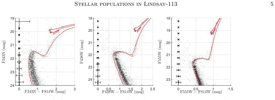
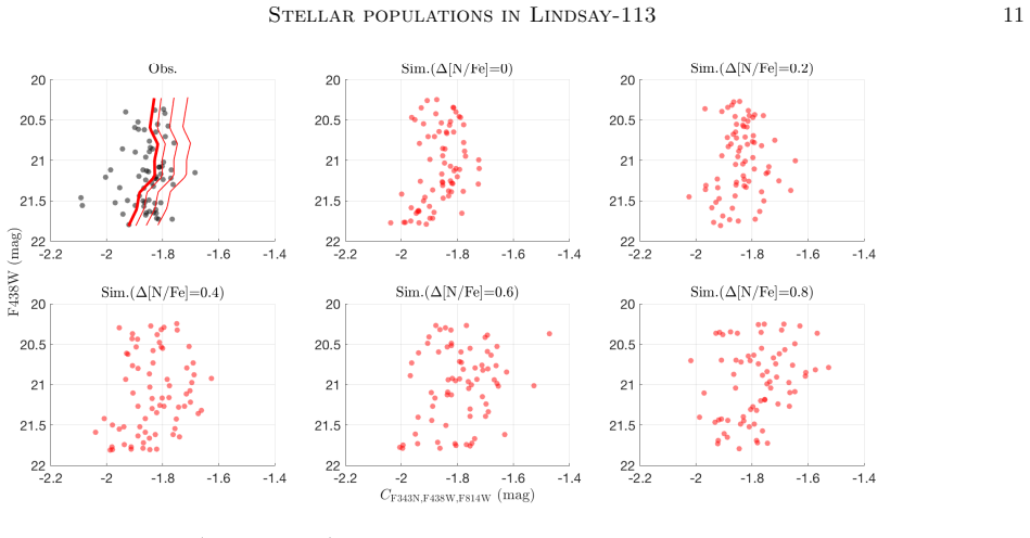
The load-bearing object is the pseudo-color index $C_{\rm F343N,F438W,F814W}=(F343N-F438W)-(F438W-F814W)$, a combination of ultraviolet, blue, and near-infrared magnitudes that highlights carbon and nitrogen abundance differences because F343N covers the NH absorption band and F438W covers the CH band. The comparison side is built from artificial stars placed on a MIST stellar-evolution isochrone and reduced through the same HST images, with an extra photometric scatter term and a differential-reddening map derived from the scatter of about 1000 main-sequence stars. Synthetic spectra from MARCS model atmospheres translate ridgeline shifts into nitrogen-abundance offsets, and repeated two-sample Kolmogorov–Smirnov tests decide which simulated populations, with $\Delta[{\rm N}/{\rm Fe}]=0.0$, 0.2, 0.4, 0.6, and 0.8 dex, are statistically consistent with the observed pseudo-color distribution.

What would settle it

Measure nitrogen abundances from high-resolution spectra of a dozen or more Lindsay 113 red giants; finding a star-to-star nitrogen spread larger than 0.2 dex would refute the paper's conclusion. Alternatively, an independent differential-reddening map obtained with a different method that yields $\delta E(B-V)\gtrsim0.01$ mag would weaken the noise explanation.

Watch

Extended reading notes

Core claim

On the paper's own terms, the discovery is that the red-giant branch of Lindsay 113 is as narrow as a single stellar population's, once all known noise sources are modeled. The authors construct the pseudo-color $C_{\rm F343N,F438W,F814W}=(F343N-F438W)-(F438W-F814W)$, which reacts to carbon and nitrogen variations, and compare its observed spread against artificial-star simulations built from the best-fitting MIST isochrone. With an assumed differential reddening of $\delta E(B-V)=0.005\pm0.002$ mag and an additional $0.003$ mag scatter per passband, the observed pseudo-color dispersion, $\sigma=0.07\pm0.02$ mag, matches the simulated simple-population value $\sigma=0.08\pm0.02$ mag; after empirically correcting the differential reddening, both drop to $\sigma=0.06\pm0.02$ mag. Synthetic MARCS spectra then convert the residual width into an upper limit of $\Delta[{\rm N}/{\rm Fe}]\leq0.2$ dex. The paper presents this as evidence that Lindsay 113, at ~4.4 Gyr old and ~23,000 $M_\odot$, is a simple stellar population—contrary to an earlier study—and that the onset of multiple populations is likely set by age and mass together.

Load-bearing premise

The paper's upper limit on nitrogen spread depends on its assumed noise budget—a differential reddening of $\delta E(B-V)=0.005\pm0.002$ mag and an extra 0.003 mag scatter per passband—and if that noise is underestimated, real variations up to ~0.2 dex or more could be hiding in the red-giant width.

Editorial extensions

If this is right

If Lindsay 113 is truly a simple stellar population, a ~4.4 Gyr-old cluster can lack the nitrogen enrichment that marks most older globular clusters, so the age boundary for multiple populations is not a sharp universal cutoff.
The comparison with the more massive and nitrogen-spread cluster NGC 2121 points to a mass threshold near $3\times10^4\,M_\odot$ for the appearance of chemical spreads among intermediate-age clusters.
Earlier photometric detections of multiple populations in UV passbands that did not correct for differential reddening may need re-examination, since a reddening of only $\delta E(B-V)\sim0.005$ mag mimics a spread of several tenths of a dex in nitrogen.
Lindsay 113 becomes a calibrator for simple-stellar-population models of intermediate-age clusters, useful for testing stellar evolution and cluster formation at lower masses.
Future surveys of 2–6 Gyr-old clusters should measure differential reddening with main-sequence stars before using red-giant widths to claim chemical complexity.

Reading between the lines

Editorial extensions of the paper, not claims the author makes directly.

A decisive, cheap extension is high-resolution spectroscopy of roughly 10–20 Lindsay 113 red giants: if the true nitrogen spread is below 0.2 dex, the photometric upper limit is validated; if above, the noise model is wrong.
The same pseudo-color method applied to the other low-mass, intermediate-age clusters in the Magellanic Clouds could map the mass boundary far more sharply, and might reveal that several previous detections of multiple populations were reddening artifacts.
The result implies that a cluster's total mass may set the number of polluting stars available during early formation, so simple stellar populations should be common below a few tens of thousands of solar masses regardless of age—a prediction testable with the next generation of large telescopes.
If age were the sole controller, Lindsay 113 should have shown multiple populations because it is older than 2 Gyr; its homogeneity is therefore indirect evidence that self-enrichment requires a minimum cluster mass, not merely time.

Share X Bluesky LinkedIn Reddit HN

Signed reviews

No signed human review yet.

Editorial analysis

A structured set of objections, weighed in public.

Desk editor's note, referee report, and a circularity audit.

Desk Editor's Note

read the letter

Li et al. present HST photometry of the SMC cluster Lindsay 113 and argue that its red-giant-branch width in a C,N-sensitive pseudo-color index is consistent with a simple stellar population, putting an upper limit of Delta[N/Fe] <= 0.2 dex. That directly contradicts Martocchia et al. (2019), who reported multiple populations in the same cluster. The best part is the independent reddening correction: using the Milone et al. (2012) method on F336W-F814W, they build a differential-reddening map and show that after correction the observed RGB width matches the artificial-star width, both at sigma ~ 0.06 mag. The bootstrap K-S comparisons are a sensible way to handle the small 67-star RGB sample. The soft spots are substantial. First, the differential-reddening noise is overestimated. In Section 4.1, they calculate the reddening contribution to the Martocchia color index by adding per-band errors in quadrature, getting delta_C ~ 0.045 mag. But differential reddening moves a star along a single reddening vector; the correct spread in a linear color index is the coherent sum of coefficients times sigma_E, roughly 0.006-0.009 mag for delta_E(B-V)=0.005. More telling, the same mistake seems to enter the Section 3.2 simulations: adding coherent reddening to their primary pseudo-color would increase the width by only ~0.01 mag, yet their simulated SSP width jumps from 0.06 to 0.08 mag. That is what independent per-band Gaussian noise would produce. So the synthetic RGB used for the K-S upper limit is too broad, and the <=0.2 dex constraint is not solid. Second, the K-S test section is written backward. They say H=0 means the null hypothesis is rejected and the distributions are the same, which is not how the test works. The table numbers make clear that H=1 is meant to indicate consistency, but as written the statistical claim is confusing and needs to be fixed. Third, the F336W data used for the reddening correction is never described in the data reduction section; they need to state where those photometry come from and how they were reduced. The qualitative conclusion that Lindsay 113 shows no strong sign of multiple populations may survive a correct noise model, since the reddening-corrected widths do match SSP predictions. But the quantitative upper limit depends on the flawed propagation. This is worth a serious referee, but only after major revision.

Referee Report

3 major / 4 minor

Summary. The paper presents HST photometry of the intermediate-age (4.37 +/- 0.20 Gyr), low-mass (~23,000 Msun) Small Magellanic Cloud cluster Lindsay 113 and asks whether the width of its red-giant branch in a nitrogen-sensitive pseudo-color index, CF343N,F438W,F814W = (F343N-F438W)-(F438W-F814W), can be explained by a simple stellar population with photometric noise, artifacts, and differential reddening. Using artificial-star tests and synthetic spectra, the authors conclude that the observed RGB width is consistent with an SSP and that any internal nitrogen spread does not exceed Delta[N/Fe] = 0.2 dex. This contradicts a previous detection of multiple populations in the same cluster by Martocchia et al. (2019). The paper includes an independent differential-reddening correction based on the F336W vs F336W-F814W CMD, which supports the adopted reddening amplitude, and discusses the implications for the age-mass parameter space of multiple populations.

Significance. If the conclusion holds, Lindsay 113 is a rare, well-observed intermediate-age, low-mass SSP, providing an important benchmark for the debate on whether age or mass controls the onset of multiple stellar populations. The paper is significant because it directly challenges a recent MP detection in the same object and offers a plausible resolution via differential reddening. The independent differential-reddening correction in Section 3.3, the use of a large artificial-star sample, and the bootstrap uncertainties on the RGB width are genuine strengths. However, the statistical analysis in Section 3.4 and the reddening propagation in Section 4.1 contain errors that must be corrected before the central claim is fully supported; the significance is therefore conditional on these revisions.

major comments (3)

[Section 3.4, Table 1] The description and use of the K-S test statistic H are internally inconsistent and contrary to standard conventions. The text states that H=0 means 'the null hypothesis is rejected, indicating that the observed and simulated ... are drawn from the same distribution,' which is incoherent, and then Table 1 reports N(H=1)=9084 for the SSP as evidence that the SSP reproduces the observation. In the standard two-sample K-S test, H=1 means the null hypothesis (same underlying distribution) is rejected, while H=0 means failure to reject; with an average P=0.31 the null should not be rejected, so the reported H values are inverted relative to the P values. As written, the H column contradicts the P column, and the conclusion that Delta[N/Fe] <= 0.2 dex is not reliably supported. The authors must correct the definitions, rerun or relabel the test, and restate the upper-limit conclusion using a correctly interpreted test.
[Section 4.1 and Section 3.2] The propagation of differential reddening into the color index treats the per-passband reddening displacements as independent random errors. For a coherent reddening vector, a linear color index C = sum c_i m_i has a spread given by |sum c_i k_i| R_V sigma_E, not sqrt(sum c_i^2 k_i^2) R_V sigma_E. For the index C' = (F343N-F438W)-(F438W-F336W), using the announced coefficients k_343=k_336=1.6 and k_438=1.3, the coherent shift for delta E(B-V)=0.005 mag is about 0.009 mag, roughly a factor of five smaller than the claimed 0.045 mag. The same issue may affect the simulated SSP widths in Section 3.2 if the adopted delta E was added as independent per-band noise. The quantitative statement in Section 4.1 that differential reddening fully explains the Martocchia et al. width is therefore not valid as it stands. The simulated widths should be recomputed with coherent reddening; based on the observed sigma=0.07 +/- 0.02 and the reddening-free AS width sigma=0.06 +/- 0.02, the central conclusion may still survive, but the present derivation is incorrect.
[Section 3.2 and Section 3.4] The noise budget used to build the synthetic SSPs is partly tuned: delta E(B-V)=0.005 +/- 0.002 mag is selected by matching the simulated CMD width to the observed width, and the additional per-band scatter delta=0.003 mag is adopted from previous work. The independent differential-reddening correction in Section 3.3 provides valuable support for the adopted delta E, but the upper limit on Delta[N/Fe] in Section 3.4 is still conditional on this partly tuned noise model. The authors should state this limitation explicitly and, ideally, present the abundance upper limit as a function of the assumed noise parameters, so readers can judge how much chemical spread could be hidden if the true noise were larger.

minor comments (4)

[Equations (1)-(4)] The fitted functions use the form P(Delta C) = A exp[-(Delta C/sigma)^2], but the quoted 'internal spread at 68% confidence' is then labeled sigma. For a Gaussian distribution, the standard deviation is sigma/sqrt(2), not the exponent parameter sigma; please clarify the convention used.
[Section 3.4] The null hypothesis of the two-sample K-S test is that the two samples are drawn from the same continuous distribution, not that they are 'independent.' Independence is not what the test assesses, and the statement should be corrected.
[Table 1] The column heading 'N (H = 1)' should be accompanied by an unambiguous definition of H and by a clear statement that average P values are reported; as shown, the H and P columns are mutually contradictory under standard conventions.
[Abstract and Section 4.2] The abstract states 'no evidence of multiple stellar populations' while the quantified conclusion is an upper limit of Delta[N/Fe] <= 0.2 dex; phrasing such as 'no evidence above 0.2 dex' would be more precise.

Circularity Check

1 steps flagged · score 4.0 of 10

Differential-reddening amplitude is fitted from the observed CMD width and then reused in the SSP comparison, but an independent reddening-correction path keeps the central claim from reducing entirely to that fit.

fitted input called prediction [Section 3.2 (Synthetic SSPs), used again in Section 3.3 (Statistical Analyses)]
"We then compare the width of the observed RGB with that of the simulation with differential reddening (see Section 3.3 for the identification of the RGB). We conclude that the degree of differential reddening is most likely δE(B − V ) = 0.005 ± 0.002 mag. ... We find that the observed distribution of ∆ CF343N,F438W,F814W for RGB stars is well consistent with that of the simulations, i.e., SSPs."

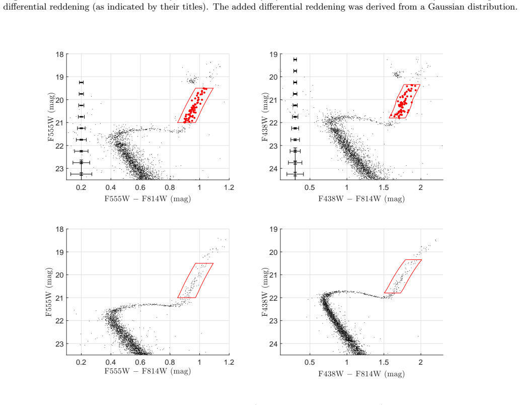
The reddening parameter δE(B−V)=0.005 mag is calibrated by matching the observed excess CMD broadening relative to reddening-free simulations, and the same value is then injected into the SSP simulations whose RGB width is compared with the observations. The claimed consistency between the observed RGB width and the SSP model is therefore partly guaranteed by construction: the noise budget was tuned to absorb the observed dispersion. The circularity is only partial because Section 3.3 provides an independent differential-reddening correction based on MS-star residuals and repeats the comparison on reddening-corrected data, obtaining σ=0.06 mag for both observation and simulations, which does not rely on the fitted δE value.

full rationale

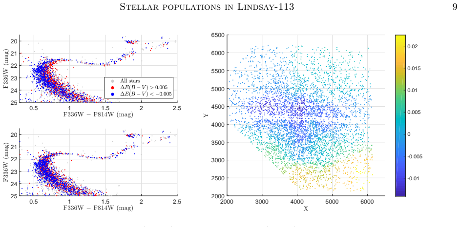
The main non-circular path is the reddening-corrected analysis: using the Milone et al. (2012) method on ~1000 MS stars, the authors derive a per-star differential-reddening map from neighbor residuals, correct the RGB, and compare it with ASs that are free of differential reddening. Both give σ=0.06±0.02 mag, independently supporting the SSP interpretation and the Δ[N/Fe]≤0.2 limit. The earlier adoption of δE(B−V)=0.005 mag is an empirical fit to the observed broadening, and reusing it in the Section 3.3 simulation comparison is a mild fitted-input-called-prediction element, but it is not the sole support for the conclusion. No load-bearing uniqueness theorem or self-citation chain is present: the 0.003 mag per-passband extra noise is cited to Milone et al. (2012), an external empirical calibration, and the Li & de Grijs (2019) citation is used as a contrast case, not as support for Lindsay 113. The score of 4 reflects the fitted reddening reuse while acknowledging that the central claim survives through an independent reddening-correction path.

Assumptions & free parameters 6 free parameters · 4 assumptions · 0 invented entities

The analysis assumes standard stellar models, a CNO-conservation enrichment pattern, and a specifically tuned noise model. No new physical entities are introduced. The free parameters are cluster parameters from isochrone fits plus the reddening/noise budget; the differential reddening and extra noise directly control the null result.

free parameters (6)

cluster age = log t = 9.64 ± 0.02 yr (4.37 ± 0.20 Gyr)
Determined by isochrone fit to the subgiant branch; used to select the synthetic isochrone and artificial stars.
metallicity [Fe/H] = -1.15 ± 0.10 dex
Inferred from the RGB slope; adopted in the isochrones and synthetic spectra.
distance modulus (m-M)0 = 18.78 ± 0.05 mag
Set from the red clump position; fixes the absolute photometric scale.
foreground reddening E(B-V) = 0.05 ± 0.01 mag
Set from the red clump position; adopted as the mean reddening.
differential reddening δE(B-V) = 0.005 ± 0.002 mag
Estimated by matching the broadening of the observed CMD; directly affects whether the RGB width can be explained by noise alone.
additional per-band noise δ = 0.003 mag
Adopted from Milone et al. 2012 and added to each passband in the artificial-star simulations; inflates the SSP width and thus weakens the limit on real nitrogen spread.

assumptions (4)

domain assumption MIST isochrones and MARCS model atmospheres accurately represent stellar evolution and spectra for this SMC cluster.
Used throughout to build synthetic CMDs and spectral loci; if these models are biased, the inferred nitrogen-spread limit shifts.
domain assumption The F343N pseudo-color index is primarily a nitrogen-abundance diagnostic, and enriched stars conserve total CNO.
Section 3.1 sets Δ[(C+N+O)/Fe]=0 and maps CNO changes to color changes; the entire detection method depends on this mapping.
domain assumption Lindsay 113 is a single-age, single-metallicity simple stellar population apart from possible light-element variations.
Adopted when building synthetic CMDs; if significant field-star contamination or age spread is present, the RGB width interpretation changes.
domain assumption The differential-reddening correction using MS fiducials and 45 neighboring stars is reliable.
Section 3.3; the reddening-free comparison and the final Δ[N/Fe] limit inherit any systematic error in this correction.

how reviews work

0 comments

Cite this review

Pith. "Pith review of When does the onset of multiple stellar populations in star clusters occur-II: No evidence of multiple stellar populations in Lindsay 113." pith.science (2026). https://pith.science/paper/KW2C6ARR

@misc{pith2026190807200,
  author       = {Pith},
  title        = {Pith review of: When does the onset of multiple stellar populations in star clusters occur-II: No evidence of multiple stellar populations in Lindsay 113},
  year         = {2026},
  howpublished = {\url{https://pith.science/paper/KW2C6ARR}},
  note         = {Machine review of arXiv:1908.07200}
}

abstract

The presence of multiple populations (MPs) in almost all globular clusters (GCs) older than ~10 Gyr, has caught lots of attention. Recently, cumulative evidence indicates that extragalactic GCs that are older than 2 Gyr, seem to also harbor MPs, however, those that are younger than 2 Gyr do not. These observations seem to imply that age is a primary property that controls the presence of MPs in star clusters. However, because of the lack of studies of {intermediate-age (~2--6 Gyr-old),} low mass clusters, it is unclear if the cluster mass, in addition to age, also plays a role in the occurrence of MPs. In this work, we studied a $\sim$4 Gyr-old, low mass (~23,000 Msun) cluster, Lindsay-113, in the Small Magellanic Cloud. Using Hubble Space Telescope photometry, we find that the width of the red-giant branch in this cluster, when measured in a specific color index that is sensitive to star-to-star chemical variations, {can be adequately explained by a "simple" stellar population model with some possible noises contributed from measurement uncertainty, photometric artifact, as well as differential reddening. The comparison of observations with predictions from synthetic spectra indicates that the internal chemical spread in nitrogen abundance, which is a signature of MPs, would not exceed 0.2 dex. Since Lindsay 113 is significantly older than other GCs with MPs, we suggest that the onset of MPs is likely determined by the combination of cluster age and mass.

Figures

Figures reproduced from arXiv: 1908.07200 by the authors.

**Figure 1.** Top: Model spectra of different CNO composition. The blue spectrum represents the star of normal abundances, while the red one represents the star of enhanced nitrogen and depleted carbon and oxygen (∆[N/Fe] = +0.8 dex, ∆[C/Fe] = ∆[O/Fe] = -0.4 dex). The stellar parameters are indicated at the right-bottom corner. Bottom: Flux ratio and filter transmission curves used here (from left to right: F343N/WFC3, F438W/WFC3… view at source ↗

**Figure 2.** Lindsay 113 CMDs. (left) F343N−F814W vs F343N; (middle) F438W−F814W vs F438W; (right) F555W−F814W vs F555W. Red lines are best-fitting isochrones. In each panel, average photometric uncertainties (corresponding to 90% confidence interval) are on the left side. any conclusion on the presence of multiple populations in Lindsay 113 (or any other cluster) should account for these properties of ASs. Recently Martocchia e… view at source ↗

**Figure 3.** The observed CMD of Lindsay 113 with error bars (left) and simulated CMDs characterized by different degrees of differential reddening (as indicated by their titles). The added differential reddening was derived from a Gaussian distribution. 0.2 0.4 0.6 0.8 1 1.2 18 19 20 21 22 23 0.5 1 1.5 2 19 20 21 22 23 24 0.2 0.4 0.6 0.8 1 1.2 18 19 20 21 22 23 0.5 1 1.5 2 19 20 21 22 23 24 [PITH_FULL_IMAGE:figures/full_fig_p0… view at source ↗

Figures from the paper (9 more)

**Figure 4.** Figure 4: Identification of RGB stars from the observations (with error bars on the left side). Stars located in selection boxes of both CMDs involving F438W, F555W and F814W are member RGB stars. The selection boxes were determined based on the artificial CMDs (bottom panels). …

**Figure 5.** Figure 5: The CF343N,F438W,F814W vs. F438W diagram for the observation with error bars (first row, left panel), the red dots are selected RGB stars. Other panels exhibit eight examples of simulated SSPs this internal spread of the pseudo-color index (corresponding to a 68% conf…

**Figure 6.** Figure 6: Left: the observed distributions of ∆CF343N,F438W,F814W (red circles) versus that for the simulations (blue circles). The red and blue curves are their best fitting Gaussian curves. Right: the observed histogram for stars with different ∆CF343N,F438W,F814W. The black …

**Figure 7.** Figure 7: Left-top: CMDs of stars with ∆E(B − V ) > 0.005 mag and ∆E(B − V ) < −0.005 mag. Left-bottom: CMDs of stars with ∆E(B − V ) > 0.005 mag and ∆E(B − V ) < −0.005 mag, with differential reddening effect corrected. Right: the differential reddening map (∆E(B − V ) (mag)) f…

**Figure 8.** Figure 8: Similar to [PITH_FULL_IMAGE:figures/full_fig_p009_8.png]

**Figure 9.** Figure 9: The same as the left panel of [PITH_FULL_IMAGE:figures/full_fig_p010_9.png]

**Figure 10.** Figure 10: The observed (top-left panel) and the simulated RGB stars with different CNO abundances in the CF343N,F438W,F814W versus F438W diagram. The thick solid line is the best fitting ridgeline to the observation. From left to right, the thin solid lines are loci with ∆[N/Fe…

**Figure 11.** Figure 11: The ∆CF 336W,F 438W,F 343N distribution for artificial RGB stars with/without differential reddening (red/blue histograms). cal dashed line. All clusters younger than this age range do not exhibit MPs, while most of their older counterparts do. For clusters between 2…

**Figure 12.** Figure 12: The age-mass plane for clusters with and without MPs (red circles and blue squares), and Lindsay 113 (the blue pentagram). The vertical and horizontal dashed lines indicate the possible age and mass boundary which may define the presence of MPs. Grey areas were the su…

Discussion (0). Continue with ORCID to comment.

Reference graph

Works this paper leans on

69 extracted references · 43 canonical work pages

[1]

Barker, H., & Paust, N. E. Q. 2018, PASP, 130, 034204

work page 2018
[2]

2014, MNRAS, 443, 3594

Bastian, N., & Strader, J. 2014, MNRAS, 443, 3594

work page 2014
[3]

2015, MNRAS, 449, 3333

Bastian, N., Cabrera-Ziri, I., & Salaris, M. 2015, MNRAS, 449, 3333

work page 2015
[4]

2018, ARA&A, 56, 83

Bastian, N., & Lardo, C. 2018, ARA&A, 56, 83

2018
[5]

Baumgardt, H., Parmentier, G., Anders, P., & Grebel, E. K. 2013, MNRAS, 430, 676

2013
[6]

A., Dickens, R

Bell, R. A., Dickens, R. J., & Gustafsson, B. 1979, ApJ, 229, 604

work page 1979
[7]

2014, A&A, 569, A111

Blanco-Cuaresma, S., Soubiran, C., Heiter, U., & Jofr´ e, P. 2014, A&A, 569, A111

2014
[8]

2019, MNRAS, 486, 2075

Blanco-Cuaresma, S. 2019, MNRAS, 486, 2075

2019

Show all 69 references

[9]

2017, A&A, 607, A44

Bragaglia, A., Carretta, E., D’Orazi, V., et al. 2017, A&A, 607, A44

2017
[10]

M., Bell, R

Briley, M. M., Bell, R. A., Smith, G. H., & Hesser, J. E. 1989, ApJ, 341, 800

1989
[11]

D., Croke, B

Cannon, R. D., Croke, B. F. W., Bell, R. A., Hesser, J. E., & Stathakis, R. A. 1998, MNRAS, 298, 601

1998
[12]

G., et al

Carretta, E., Bragaglia, A., Gratton, R. G., et al. 2009, A&A, 505, 117

2009
[13]

G., et al

Carretta, E., Bragaglia, A., Gratton, R. G., et al. 2010, A&A, 516, A55

2010
[14]

M., Sweigart, A

Cavallo, R. M., Sweigart, A. V., & Bell, R. A. 1996, ApJL, 464, L79

1996
[15]

M., Sweigart, A

Cavallo, R. M., Sweigart, A. V., & Bell, R. A. 1998, ApJ, 492, 575

1998
[16]

2019, MNRAS, 484, 5236

Chantereau, W., Salaris, M., Bastian, N., & Martocchia, S. 2019, MNRAS, 484, 5236

2019
[17]

2016, ApJ, 823, 102

Choi, J., Dotter, A., Conroy, C., et al. 2016, ApJ, 823, 102

2016
[18]

P., Marino, A

Cordoni, G., Milone, A. P., Marino, A. F., et al. 2018, ApJ, 869, 139

2018
[19]

2016, ApJ, 829, 77 D’Antona, F., Milone, A

Dalessandro, E., Lapenna, E., Mucciarelli, A., et al. 2016, ApJ, 829, 77 D’Antona, F., Milone, A. P., Tailo, M., et al. 2017, Nature Astronomy, 1, 0186

2016
[20]

2007, A&A, 464, 1029 D’Ercole, A., Vesperini, E., D’Antona, F., McMillan, S

Decressin, T., Meynet, G., Charbonnel, C., Prantzos, N., & Ekstr¨ om, S. 2007, A&A, 464, 1029 D’Ercole, A., Vesperini, E., D’Antona, F., McMillan, S. L. W., & Recchi, S. 2008, MNRAS, 391, 825 de Mink, S. E., Pols, O. R., Langer, N., & Izzard, R. G. 2009, A&A, 507, L1 Dolphin A...

2007
[21]

2018, ApJL, 865, L10

Sarajedini, A. 2018, ApJL, 865, L10

2018
[22]

K., Dotter, A., Johnson, C

Dupree, A. K., Dotter, A., Johnson, C. I., et al. 2017, ApJL, 846, L1

2017
[23]

2017, MNRAS, 468, L11

For, B.-Q., & Bekki, K. 2017, MNRAS, 468, L11

2017
[24]

2019, A&A, 622, A66

Georgy, C., Charbonnel, C., Amard, L., et al. 2019, A&A, 622, A66

2019
[25]

O., & Corbally, C

Gray, R. O., & Corbally, C. J. 1994, AJ, 107, 742

1994
[26]

2008, A&A, 486, 951

Gustafsson, B., Edvardsson, B., Eriksson, K., et al. 2008, A&A, 486, 951

2008
[27]

2019, MNRAS, 484, 4718

Hollyhead, K., Martocchia, S., Lardo, C., et al. 2019, MNRAS, 484, 4718

2019
[28]

2017, MNRAS, 472, 67

Hong, J., de Grijs, R., Askar, A., et al. 2017, MNRAS, 472, 67

2017
[29]

2014, ApJ, 789, 88

Jiang, D., Han, Z., & Li, L. 2014, ApJ, 789, 88

2014
[30]

Krause, M. G. H., Charbonnel, C., Bastian, N., & Diehl, R. 2016, A&A, 587, A53

2016
[31]

P., Milone, A

Lagioia, E. P., Milone, A. P., Marino, A. F., & Dotter, A. 2019, ApJ, 871, 140 14 Li et al

2019
[32]

S., Brodie, J

Larsen, S. S., Brodie, J. P., Grundahl, F., & Strader, J. 2014, ApJ, 797, 15

2014
[33]

2006, A&A, 453, 547

Letarte, B., Hill, V., Jablonka, P., et al. 2006, A&A, 453, 547

2006
[34]

2016, Nature, 529, 502

Li, C., de Grijs, R., Deng, L., et al. 2016, Nature, 529, 502

2016
[35]

Li, C., de Grijs, R., Deng, L., & Milone, A. P. 2017, ApJ, 844, 119

2017
[36]

2019, ApJ, 876, 94

Li, C., & de Grijs, R. 2019, ApJ, 876, 94

2019
[37]

F., Villanova, S., Piotto, G., et al

Marino, A. F., Villanova, S., Piotto, G., et al. 2008, A&A, 490, 625

2008
[38]

F., Milone, A

Marino, A. F., Milone, A. P., Piotto, G., et al. 2009, A&A, 505, 1099

2009
[39]

F., Przybilla, N., Milone, A

Marino, A. F., Przybilla, N., Milone, A. P., et al. 2018, AJ, 156, 116

2018
[40]

F., Milone, A

Marino, A. F., Milone, A. P., Casagrande, L., et al. 2018, ApJL, 863, L33

2018
[41]

2017, MNRAS, 468, 3150

Martocchia, S., Bastian, N., Usher, C., et al. 2017, MNRAS, 468, 3150

2017
[42]

2018, MNRAS, 473, 2688

Martocchia, S., Cabrera-Ziri, I., Lardo, C., et al. 2018, MNRAS, 473, 2688

2018
[43]

2019, MNRAS

Martocchia, S., Dalessandro, E., Lardo, C., et al. 2019, MNRAS

2019
[44]

E., & van der Marel, R

McLaughlin, D. E., & van der Marel, R. P. 2005, ApJS, 161, 304

2005
[45]

P., Bedin, L

Milone, A. P., Bedin, L. R., Piotto, G., & Anderson, J. 2009, A&A, 497, 755

2009
[46]

P., Piotto, G., Bedin, L

Milone, A. P., Piotto, G., Bedin, L. R., et al. 2012, A&A, 540, A16

2012
[47]

P., Piotto, G., Renzini, A., et al

Milone, A. P., Piotto, G., Renzini, A., et al. 2017, MNRAS, 464, 3636

2017
[48]

P., Marino, A

Milone, A. P., Marino, A. F., Renzini, A., et al. 2018, MNRAS, 481, 5098

2018
[49]

P., Stetson, P

Monelli, M., Milone, A. P., Stetson, P. B., et al. 2013, MNRAS, 431, 2126

2013
[50]

R., & Pancino, E

Mucciarelli, A., Origlia, L., Ferraro, F. R., & Pancino, E. 2009, ApJL, 695, L134

2009
[51]

R., Origlia, L., & Lanzoni, B

Mucciarelli, A., Dalessandro, E., Ferraro, F. R., Origlia, L., & Lanzoni, B. 2014, ApJL, 793, L6

2014
[52]

2017, MNRAS, 465, 4159

Niederhofer, F., Bastian, N., Kozhurina-Platais, V., et al . 2017, MNRAS, 465, 4159

2017
[53]

2017, A&A, 601, A112

Pancino, E., Romano, D., Tang, B., et al. 2017, A&A, 601, A112

2017
[54]

2011, ApJS, 192, 3

Paxton, B., Bildsten, L., Dotter, A., et al. 2011, ApJS, 192, 3

2011
[55]

2013, ApJS, 208, 4

Paxton, B., Cantiello, M., Arras, P., et al. 2013, ApJS, 208, 4

2013
[56]

2015, ApJS, 220, 15

Paxton, B., Marchant, P., Schwab, J., et al. 2015, ApJS, 220, 15

2015
[57]

Piatti, A. E. 2018, AJ, 156, 206

2018
[58]

A., Sneden, C., Kraft, R

Pilachowski, C. A., Sneden, C., Kraft, R. P., & Langer, G. E. 1996, AJ, 112, 545

1996
[59]

P., Bedin, L

Piotto, G., Milone, A. P., Bedin, L. R., et al. 2015, AJ, 149, 91

2015
[60]

R., Anderson, J., et al

Piotto, G., Bedin, L. R., Anderson, J., et al. 2007, ApJL, 661, L53

2007
[61]

2007, A&A, 465, 815

Sbordone, L., Bonifacio, P., Buonanno, R., et al. 2007, A&A, 465, 815

2007
[62]

J., Westmoquette, M

Smith, L. J., Westmoquette, M. S., Gallagher, J. S., et al. 2006, MNRAS, 370, 513

2006
[63]

Sun, W., de Grijs, R., Deng, L., & Albrow, M. D. 2019, ApJ, 876, 113

2019
[64]

V., & Mengel, J

Sweigart, A. V., & Mengel, J. G. 1979, ApJ, 229, 624 Tautvaiˇ sien˙ e, G., Wallerstein, G., Geisler, D., Gonzalez, G., & Charbonnel, C. 2004, AJ, 127, 373

1979
[65]

R., et al

Villanova, S., Piotto, G., King, I. R., et al. 2007, ApJ, 663, 296

2007
[66]

2013, ApJ, 778, 186

Villanova, S., Geisler, D., Carraro, G., Moni Bidin, C., & Mu˜ noz, C. 2013, ApJ, 778, 186

2013
[67]

2017, A&A, 607, A135

Wang, Y., Primas, F., Charbonnel, C., et al. 2017, A&A, 607, A135

2017
[68]

2013, ApJ, 776, 112

Yang, W., Bi, S., Meng, X., & Liu, Z. 2013, ApJ, 776, 112

2013
[69]

2018, ApJ, 853, 186

Zhang, H., de Grijs, R., Li, C., & Wu, X. 2018, ApJ, 853, 186

2018

Pith tools

Reviewed August 14, 2026 · model on record in the stance chip above.

[1] [1]

Barker, H., & Paust, N. E. Q. 2018, PASP, 130, 034204

work page 2018

[2] [2]

2014, MNRAS, 443, 3594

Bastian, N., & Strader, J. 2014, MNRAS, 443, 3594

work page 2014

[3] [3]

2015, MNRAS, 449, 3333

Bastian, N., Cabrera-Ziri, I., & Salaris, M. 2015, MNRAS, 449, 3333

work page 2015

[4] [4]

2018, ARA&A, 56, 83

Bastian, N., & Lardo, C. 2018, ARA&A, 56, 83

2018

[5] [5]

Baumgardt, H., Parmentier, G., Anders, P., & Grebel, E. K. 2013, MNRAS, 430, 676

2013

[6] [6]

A., Dickens, R

Bell, R. A., Dickens, R. J., & Gustafsson, B. 1979, ApJ, 229, 604

work page 1979

[7] [7]

2014, A&A, 569, A111

Blanco-Cuaresma, S., Soubiran, C., Heiter, U., & Jofr´ e, P. 2014, A&A, 569, A111

2014

[8] [8]

2019, MNRAS, 486, 2075

Blanco-Cuaresma, S. 2019, MNRAS, 486, 2075

2019