REVIEW 5 minor 1 cited by
Computing the Stable Reduction of Hyperelliptic Curves in Residue Characteristic 2
T0 review · 0 major / 5 minor · reviewed 2026-08-15 · deepseek-v4-flash
Pith's one-line read This paper proves two closed-form formulas for the local genus of the stable reduction of a hyperelliptic curve in residue characteristic 2, and shows how they make explicit computation practical up to genus 30.
desk verdict A genuine continuation of the square-defect program with checkable local-genus formulas; black-box dependence on two prior propositions is the main risk, not the paper's own proofs. read the letter →
The pith
A machine-rendered reading of the paper's core claim, the machinery that carries it, and where it could break.
The reading
What carries the argument
The central object is the square defect $w(F)$, defined as the minimum of $2$ and the largest valuation of $F - H^2$ over all Laurent polynomials $H$; it measures how closely $F$ can be approximated by a square. At a double point this becomes the piecewise-linear square defect function $w_{\bar p,X}(\lambda) = w(F(2^{\lambda}u))$, whose break points correspond to components of the base model and whose slopes encode genera. The argument runs through optimal decompositions $F = H^2 + G$ and the explicit local equations of the normalization from [10, Prop. 3.3.2], which is what turns the two formulas into actual computations.
What would settle it
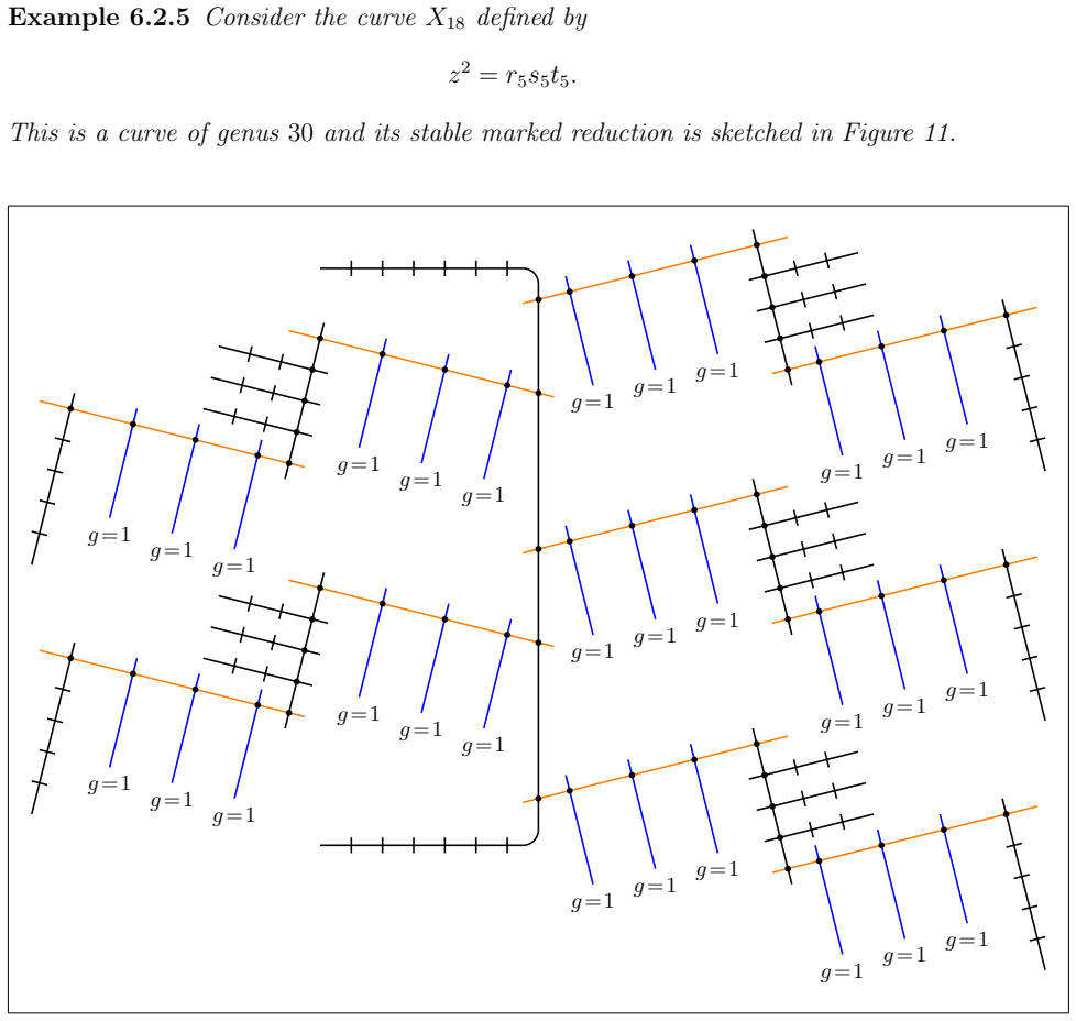
Recompute the stable marked reduction of $X_{18}$ (genus 30, $z^2 = r_5 s_5 t_5$) by the full normalization algorithm of [10] without the shortcuts, and compare the resulting components and genera with the paper's Figure 11; a mismatch in any local genus over a smooth point or even double point refutes Theorems 4.2.2 and 4.3.1. A smaller check: for a curve with known $F$, compute the root multiplicity of $[dG/dx/2^{\gamma}]$ directly and compare it with the genus of the Artin-Schreier component obtained from [10, Prop. 3.3.2].
Extended reading notes
Core claim
The central discovery is that the hard local information in the stable reduction is carried by two formulas. If $F = H^2 + G$ is an optimal decomposition of a Weierstrass equation and $\gamma := w(F) < 2$, then the local genus over a smooth unmarked point $\bar p$ is half the multiplicity of the root of $[dG/dx/2^{\gamma}]$ at $\bar p$ (Theorem 4.2.2). Over an even double point, writing $s_1$ and $s_2$ for the largest and smallest slopes of the square defect function $w_{\bar p,X}$, the local genus is $(s_1 - s_2 + \delta_{0s_1} + \delta_{0s_2})/2$ (Theorem 4.3.1). These formulas, together with the grounded-double-point criteria and leaf-component bounds, convert a substantial part of stable reduction into elementary arithmetic on a single Laurent polynomial and its derivative.
Load-bearing premise
Everything rests on the square-defect machinery of [10], above all the explicit local equations for the normalization and the statement that break points of the square defect function correspond to components of the base model; if either of those results were false, the two local-genus theorems would not be established.
Editorial extensions
If this is right
- Because $F$ can be replaced by any Laurent polynomial $\tilde F$ that is sufficiently close in valuation, the semistable normalization above a smooth point or even double point is unchanged; this lets one discard high-degree pieces of $F$ and avoid the high-degree stability polynomial.
- If the base curve has $g$ grounded double points, every one of them has local genus $1$, and its entire reduction is determined by the thicknesses, with the explicit structure described in Proposition 5.2.4.
- The toric rank of the reduction of the Jacobian equals the number of grounded double points of thickness strictly greater than $4$ (Corollary 5.2.7).
- For genus 3 curves with three grounded double points, 115 combinatorial types of the stable reduction are obtained, each depending only on the thicknesses of the double points.
- The curves $X_{10}, X_{11}, X_{16}, X_{17}, X_{18}$ all have toric rank $0$ in their reductions over $2$, and $X_{18}$ is the highest-genus hyperelliptic curve whose stable reduction over $2$ has been explicitly computed.
Reading between the lines
- A natural algorithmic consequence, not pursued in the paper, is to factor $[dG/dx/2^{\gamma}]$ in $k[x^2]$ early: the total local genus over a smooth component is bounded by half its degree, so a partial root count could terminate the normalization computation before all components are built.
- The leaf-component inequalities in Propositions 5.3.1 and 5.3.3 are necessary conditions on the dual graph that could be turned into an automated search for all possible dual graphs of the stable reduction for a fixed genus.
- The approximation results suggest a divide-and-conquer strategy for very high genus: approximate the Weierstrass polynomial locally at each point of the base model, compute local genera independently, and assemble the reduction; a natural stress test would be random genus-10 polynomials compared against the full algorithm of [10].
- If the local-genus formula extends to other tamely ramified double covers, derivative-root multiplicity might replace full normalization in a broader class of wild stable-reduction problems.
Signed reviews
Editorial analysis
A structured set of objections, weighed in public.
Referee Report
Summary. The paper develops tools for computing the stable marked reduction of hyperelliptic curves over a characteristic-zero field with residue characteristic 2. Building on the author's earlier joint work with Pink [10], it defines a local genus for each point of the special fiber of the quotient curve and proves two central formulas: Theorem 4.2.2 expresses the local genus over a smooth unmarked point as half the multiplicity of a root of the derivative of the square-defect approximation, and Theorem 4.3.1 expresses the local genus over an even double point in terms of the largest and smallest slopes of the square defect function. It also proves approximation lemmas that allow replacing the Weierstrass polynomial by a simpler one, a thickness bound for components of type (d), a structure theorem for grounded double points, and leaf-component inequalities. The final section applies the methods to all genus-3 combinatorial cases with three grounded double points and to five explicit curves with many automorphisms, the largest of genus 30.
Significance. If correct, the local-genus formulas provide a genuinely efficient route to the stable reduction that avoids the large stability polynomial of [10], and the genus-30 example appears to be the largest explicit stable reduction computed in residue characteristic 2. The inductive proofs of Theorems 4.2.2 and 4.3.1 are detailed and checkable, and the paper is transparent about its assumptions: Conjecture 5.4.1 is explicitly labeled as conjectural, and the computational claims are backed by worksheets [8]. The main risk is external dependence: the proofs repeatedly invoke [10, Prop. 3.3.2] and [10, Prop. 4.5.1] as black boxes, so the validity of the central theorems is conditional on those results. I found no internal inconsistency in the present manuscript, and the cited dependence is legitimate rather than circular, but a separate verification of the quoted propositions is needed for full confidence.
minor comments (5)
- [§5.2, Proposition 5.2.4] In the case α > 4 the break points of w_{p,X} should be λ = 2 and λ = α − 2; the text currently writes λ1 := 2 − α and λ2 := α − 2, and 2 − α is negative for α > 4. In the same proposition, the second sentence of part (b) says that T2 intersects the proper transform of X, but it should say the proper transform of Y.
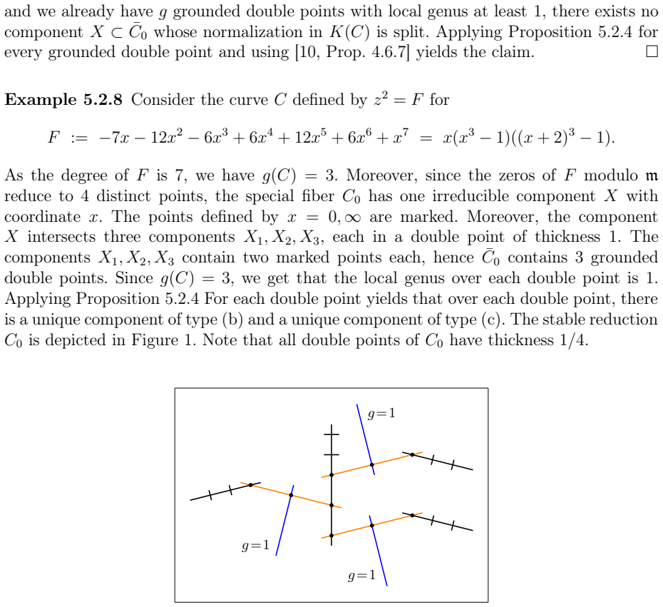
- [§5.2, Example 5.2.8] The text says that over each grounded double point there is a unique component of type (b) and a unique component of type (c); for thickness 1, Proposition 5.2.4(a)(i) gives a component of type (b) and a component of type (d), so the example should refer to type (d).
- [§4.2, proof of Theorem 4.2.2] In the induction step with a break point, the sentence 'Equations 4.2.4 and 4.2.3 yield' appears to mis-cite the line numbers: the value of s2 is defined in equation (4.2.5), so the reference should be to equations (4.2.4) and (4.2.5).
- [§5.3, Example 5.3.2(b)] The final display writes a sum over X1 in the sentence 'for each 1 ≤ i ≤ 3, we have ∑_{q∈X1} g_q = 0'; this should be a sum over Xi, and the claimed vanishing should be stated uniformly for i = 1, 2, 3.
- [§3.3, Proposition 3.3.4] The proof says that for a component of type (b) the stable reduction of C and of C̃ over the closed points of the component is isomorphic, but the proposition statement only asserts isomorphisms of the preimages of the components of types (b), (c), and (d). A brief clarification that the isomorphism is of the full preimage of the open component minus the double points would make the logical structure of the proof easier to follow.
Circularity Check
No significant circularity: the new local-genus theorems are proved from the prior square-defect machinery of [10], an external earlier work with its own proofs and computational worksheets, and no prediction reduces by definition or fitting to its inputs.
full rationale
The paper's central results, Theorems 4.2.2 and 4.3.1, are genuine new formulas for the local genus in terms of the square defect function, proved by induction from the local normal form and component-correspondence results imported from [10, Prop. 3.3.2] and [10, Prop. 4.5.1]. These imports are self-citations in the sense that the present author is also an author of [10], but they are not circular: [10] is a separate prior paper with its own proofs and accompanying worksheets, and its propositions do not already contain the local-genus formulas proved here. The paper contains no fitted parameters presented as predictions, no quantity defined in terms of the quantity it is supposed to derive, and no renaming of a known result as a new one. The dependence on the correctness of [10] is a legitimate external-dependence risk, not a circularity. Therefore the appropriate circularity score is 0.
Assumptions & free parameters
assumptions (4)
- domain assumption Correctness of square defect results from [10], e.g. Prop. 3.3.2, 3.4.4, 4.5.1, 4.5.10, 4.5.12
- standard math Standard semistable model theory: minimal semistable models, thickness of double points, blowing down, Neron model facts
- standard math Artin-Schreier genus formula for components with equations t + t^2 = P(u) or t^2 = P(u)
- standard math Separability and Hurwitz data for the double cover z^2 = F(x) in characteristic 0 with 2g + 2 ramification points
Cite this review
Pith. "Pith review of Computing the Stable Reduction of Hyperelliptic Curves in Residue Characteristic 2." pith.science (2026). https://pith.science/paper/KXPV5HPJ
@misc{pith2026250619663,
  author       = {Pith},
  title        = {Pith review of: Computing the Stable Reduction of Hyperelliptic Curves in Residue Characteristic 2},
  year         = {2026},
  howpublished = {\url{https://pith.science/paper/KXPV5HPJ}},
  note         = {Machine review of arXiv:2506.19663}
}
abstract
Consider a hyperelliptic curve of genus $g$ over a field $K$ of characteristic zero. After extending $K$ we can view it as a marked curve with its $2g+2$ Weierstrass points. We prove some general properties of the stable reduction of this marked curve for a valuation of residue characteristic $2$ and refine an existing algorithm for its computation. We work out explicit examples up to genus $g=30$.
Figures


Figures from the paper (8 more)


Forward citations
Cited by 1 Pith paper
-
Semistable reduction of smooth quartics
For smooth plane quartics, non-hyperelliptic stable reduction is equivalent to the existence of a unique GIT-stable plane model, and the stable model is obtained by cusp resolution.
Reference graph
Works this paper leans on
-
[10]
Reduction of Hyperelliptic Curves in Residue Characteristic 2
Tim Gehrunger and Richard Pink. Reduction of Hyperelliptic Curves in Residue Characteristic 2. 2024. arXiv:2404.14214 [math.AG]
arXiv 2024
-
[8]
Worksheets for this paper.url: https://doi.org/10.3929/ethz- b-000741595
Tim Gehrunger. Worksheets for this paper.url: https://doi.org/10.3929/ethz- b-000741595
-
[1]
Oxford graduate texts in mathematics
Algebraic Geometry and Arithmetic Curves. Oxford graduate texts in mathematics. Oxford University Press, 2002
work page 2002
-
[2]
Kai Arzdorf and Stefan Wewers.Another proof of the Semistable Reduction Theorem
-
[3]
Formelle Standardmodelle hyperelliptischer Kurven
Siegfried Bosch. “Formelle Standardmodelle hyperelliptischer Kurven”. In: Math. Ann. 251.1 (1980), pp. 19–42. doi: 10 . 1007 / BF01420278. url: https : / / doi . org/10.1007/BF01420278
-
[4]
Vincent Delecroix, Johannes Schmitt, and Jason van Zelm. “admcycles - a Sage package for calculations in the tautological ring of the moduli space of stable curves”. In: Journal of Software for Algebra and Geometry11.1 (Dec. 2021), pp. 89–112.doi: 10.2140/jsag.2021.11.89 . url: http://dx.doi.org/10.2140/jsag.2021.11. 89
-
[5]
Arithmetic of hyperelliptic curves over local fields
Tim Dokchitser et al. “Arithmetic of hyperelliptic curves over local fields”. In:Math. Ann. 385.3-4 (2023), pp. 1213–1322. doi: 10 . 1007 / s00208 - 021 - 02319 - y. url: https://doi.org/10.1007/s00208-021-02319-y
-
[6]
Clusters and semistable models of hyperelliptic curves in the wild case
Leonardo Fiore and Jeffrey Yelton. Clusters and semistable models of hyperelliptic curves in the wild case. 2023. arXiv:2207.12490 [math.NT]. url: https://arxiv. org/abs/2207.12490
arXiv 2023
Show all 22 references
-
[7]
Classification for the stable marked reduction of genus2 curves in residue characteristic2
Tim Gehrunger. Classification for the stable marked reduction of genus2 curves in residue characteristic2. In preparation
-
[9]
Reduction of Hyperelliptic Curves in Character- istic̸= 2
Tim Gehrunger and Richard Pink. Reduction of Hyperelliptic Curves in Character- istic̸= 2. 2021. arXiv:2112.05550 [math.AG]
2021 arXiv
-
[11]
ReductionofHyperellipticCurves in Residue Characteristic 2
TimGehrungerandRichardPink.Worksheetsfor"ReductionofHyperellipticCurves in Residue Characteristic 2".url: https://doi.org/10.3929/ethz-b-000669537
-
[12]
Arbres de Hurwitz et automorphismes d’ordre p des disques et des couronnes p-adiques formels
Y.Henrio. Arbres de Hurwitz et automorphismes d’ordre p des disques et des couronnes p-adiques formels. 2000. arXiv: math/0011098 [math.AG] . url: https://arxiv. org/abs/math/0011098
2000 arXiv
-
[13]
Wild monodromy and automorphisms of curves
Claus Lehr and Michel Matignon. “Wild monodromy and automorphisms of curves”. In: Duke Mathematical Journal135.3 (2006), pp. 569–586
2006
-
[14]
Courbes stables de genre 2 et leur schéma de modules
Qing Liu. “Courbes stables de genre 2 et leur schéma de modules”. In:Mathematische Annalen 295.1 (1993), pp. 201–222
1993
-
[15]
Hyperelliptic curves with many automorphisms
Nicolas Müller and Richard Pink. “Hyperelliptic curves with many automorphisms”. In: International Journal of Number Theory 18.04 (2022), pp. 913–930. doi: 10 . 1142/S1793042122500488.eprint: https://doi.org/10.1142/S1793042122500488. url: https://doi.org/10.1142/S1793042122500488. 43
2022 doi
-
[16]
p-groupesetréductionsemi-stabledescourbes
MichelRaynaud.“p-groupesetréductionsemi-stabledescourbes”.In: The Grothendieck Festschrift: A Collection of Articles Written in Honor of the 60th Birthday of Alexan- der Grothendieck. Ed. by Pierre Cartier et al. Boston, MA: Birkhäuser Boston, 2007, pp. 179–197. doi: 10.1007/9...
2007 doi
-
[17]
Spécialisation des revêtements en caractéristique p > 0
Michel Raynaud. “Spécialisation des revêtements en caractéristique p > 0”. fr. In: Annales scientifiques de l’École Normale Supérieure4e série, 32.1 (1999), pp. 87–
1999
-
[18]
Spécialisation du foncteur de Picard
Michel Raynaud. “Spécialisation du foncteur de Picard”. fr. In:Publications Math- ématiques de l’IHÉS 38 (1970), pp. 27–76.url: http://www.numdam.org/item/ PMIHES_1970__38__27_0/
1970
-
[19]
p-rank and semi-stable reduction of curves. II
Mohamed Saïdi. “ p-rank and semi-stable reduction of curves. II”. In:Math. Ann. 312.4 (1998), pp. 625–639.doi: 10.1007/s002080050239. url: https://doi.org/ 10.1007/s002080050239
1998 doi
-
[20]
Torsors under finite and flat group schemes of rankp with Galois action
Mohamed Saïdi. “Torsors under finite and flat group schemes of rankp with Galois action”. In:Math. Z.245.4 (2003), pp. 695–710.doi: 10.1007/s00209-003-0566-3. url: https://doi.org/10.1007/s00209-003-0566-3. 44
2003 doi
-
[126]
1016 / s0012 - 9593(99 ) 80010 - x
doi: 10 . 1016 / s0012 - 9593(99 ) 80010 - x. url: http : / / www . numdam . org / articles/10.1016/s0012-9593(99)80010-x/
-
[2012]
url: https://arxiv.org/abs/1211.4624
arXiv: 1211.4624 [math.AG]. url: https://arxiv.org/abs/1211.4624. 42
Reviewed August 15, 2026 · model on record in the stance chip above.
Discussion (0). Continue with ORCID to comment.