REVIEW 4 major objections 6 minor 46 references
Frequency selection in a gravitationally stretched capillary jet in the jetting regime
T0 review · 4 major / 6 minor · reviewed 2026-08-14 · deepseek-v4-flash
Pith's one-line read For a gravity-stretched capillary jet, the optimal forcing frequency depends strongly on forcing amplitude, and a linear resolvent analysis predicts both the frequency and the breakup length.
desk verdict Solid nonlinear study of a stretched capillary jet with an appealing but under-specified resolvent threshold criterion; worth a serious referee. read the letter →
The pith
A machine-rendered reading of the paper's core claim, the machinery that carries it, and where it could break.
The reading
What carries the argument
The central object is the resolvent gain $G_{h,f_u}(\omega,L)$ of the linearized one-dimensional slender-jet operator: the energy norm of the harmonic response in the interface height to unit inlet velocity forcing, measured in a Chebyshev-collocation energy norm with weight matrices $Q$ and $Q_f$. For each domain size $L$, the envelope $G_{\mathrm{opt}}(L)=\max_\omega G_{h,f_u}(\omega,L)$ of the dominant frequency is built; the breakup-threshold identity $G_{\mathrm{opt}}(l_c)=1/\epsilon$ then fixes the breakup length and, through the frequency at which the envelope is crossed, the optimal forcing frequency. The WKBJ amplitude equation serves as the comparison baseline: it improves the zeroth-order spatial gain but still underpredicts the gain magnitude, which is why the resolvent analysis is required for quantitative agreement.
What would settle it
Measure experimentally the breakup length and dominant drop frequency of a gravity-stretched jet with $Oh_{in}=0.3$, $We_{in}=1.75$, $Bo_{in}=0.1$ for amplitudes from $10^{-2}$ down to $10^{-8}$; the resolvent-plus-threshold predicts a monotone rise of $\omega_{\mathrm{opt}}$ and $l_c$ with no saturation, so observing a plateau or an abrupt deviation would directly falsify the criterion.
Extended reading notes
Core claim
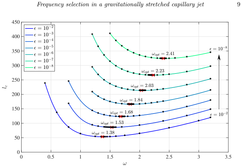
Using the one-dimensional slender-jet approximation for an axisymmetric jet with inlet parameters $Oh_{in}=0.3$, $We_{in}=1.75$, $Bo_{in}=0.1$, the authors find in nonlinear simulations that the optimal forcing frequency rises from about $1.38$ at amplitude $10^{-2}$ to about $1.68$ at $10^{-4}$, and keeps increasing without visible saturation down to $10^{-8}$, while the breakup length grows with decreasing amplitude. They then construct the dominant-frequency envelope $G_{\mathrm{opt}}(L)$ of the resolvent gain as a function of domain size and impose the order-one breakup criterion $G_{\mathrm{opt}}(l_c)=1/\epsilon$. The crossing of the envelope with the horizontal line $1/\epsilon$ selects both the breakup length $l_c$ and the amplitude-dependent optimal frequency $\omega_{\mathrm{opt}}$ without any input from nonlinear simulations, and the predicted values match the simulations. The amplitude dependence disappears when gravity is removed ($Bo_{in}=0$), where $\omega_{\mathrm{opt}}$ remains fixed as the amplitude varies, showing that the effect is caused by the gravitational stretching of the base flow. Under band-limited white-noise forcing, the jet's breakup statistics remain peaked near the quantities associated with the optimal frequency at the same amplitude.
Load-bearing premise
The load-bearing premise is that breakup happens at the downstream location where the linear response gain first reaches $1/\epsilon$; if a different threshold value or a different way of measuring the response were used, the predicted frequencies and breakup lengths would change, even though the overall trend would survive.
Editorial extensions
If this is right
- For the jet with $Oh_{in}=0.3$, $We_{in}=1.75$, $Bo_{in}=0.1$, decreasing the forcing amplitude from $10^{-2}$ to $10^{-8}$ raises both the optimal forcing frequency and the breakup length, with no saturation observed at the smallest amplitude.
- The resolvent envelope alone, with the $G_{\mathrm{opt}}(l_c)=1/\epsilon$ criterion, predicts both quantities without nonlinear simulation input; the remaining discrepancy with simulations is attributed to this threshold criterion.
- When gravity is absent ($Bo_{in}=0$), the optimal frequency is independent of amplitude, so the amplitude dependence is a distinctive consequence of gravitational stretching of the base flow.
- Under broadband white-noise forcing, the drop-size and breakup-length statistics remain centered near the values obtained with the optimal frequency at the same amplitude, implying the jet selects the amplifier-preferred mode even when forced with a broad spectrum.
- Because the jet is globally stable in the jetting regime, no self-sustained oscillations contaminate the response, so the linear resolvent is the appropriate global description of the amplification.
Reading between the lines
- The threshold constant in $G_{\mathrm{opt}}(l_c)=1/\epsilon$ is chosen ad hoc as order one; a different constant would shift $l_c$ and $\omega_{\mathrm{opt}}$ quantitatively, but any monotone threshold would preserve the qualitative rise of $\omega_{\mathrm{opt}}$ as $\epsilon$ falls.
- The same envelope-crossing construction could be applied to other spatially developing, convectively unstable flows—stretched viscous threads, electrically forced jets, or spinning fibres—wherever the base flow stretches perturbation wavelengths downstream; the amplitude-dependence of the preferred frequency would appear whenever the forcing level changes.
- The lack of saturation at $10^{-8}$ is falsifiable: experiments or simulations at even smaller amplitudes should show the optimal frequency still climbing if the mechanism is right, and saturating if a competing nonlinear selection or noise floor takes over.
- The oscillation of the breakup period between main and satellite drop groups suggests that the timing statistics, not just the mean period, carry information about the forcing frequency and could serve as a sensitive experimental probe.
Signed reviews
Editorial analysis
A structured set of objections, weighed in public.
Referee Report
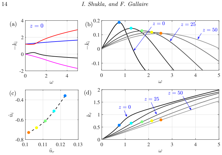
Summary. The paper investigates how the amplitude of an externally imposed harmonic inlet forcing selects the optimal frequency and breakup length of a gravitationally stretched capillary jet in the jetting regime. The authors use nonlinear simulations of the one-dimensional Eggers & Dupont equations for a jet with Ohin=0.3, Wein=1.75, Boin=0.1 and forcing amplitudes epsilon=10^-2 to 10^-8. The simulations show that lowering the forcing amplitude increases both the breakup length and the optimal forcing frequency, unlike the case Boin=0 where the optimal frequency is amplitude-independent. A local spatial and WKBJ stability analysis fails to reproduce the simulation trends quantitatively. The authors then perform a global resolvent analysis of the linearized operator of the stretched base state. They introduce the envelope G_opt(L) of the maximal resolvent gain over frequency as a function of domain length, and propose the breakup criterion G_opt(lc)=1/epsilon (Eq. 4.34). With this criterion, the resolvent analysis predicts both the optimal frequency and the breakup length as functions of epsilon, in good agreement with the nonlinear simulations (Fig. 13). The paper also compares the jet response under white-noise inlet forcing with the expected response at the optimal frequency.
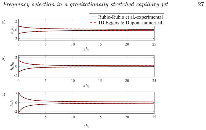
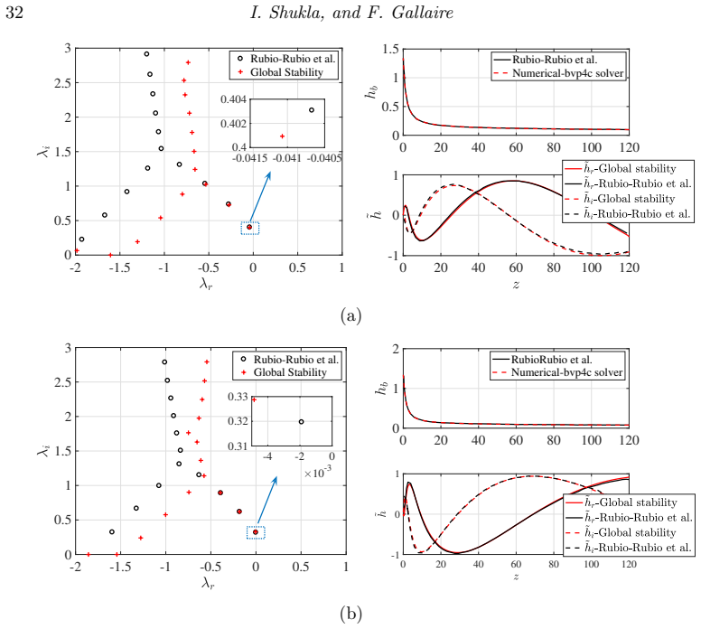
Significance. If the quantitative predictions are robust, the paper makes a useful contribution by showing that resolvent analysis, supplemented by an amplitude-dependent breakup criterion, can capture the amplitude sensitivity of the preferred frequency in a non-parallel capillary jet, a result that goes beyond the constant-noise-level WKBJ approach of Le Dizès & Villermaux (2017). The strengths of the manuscript are the careful validation of the nonlinear code against van Hoeve et al. (2010) (Appendix 7.3), of the base state and global stability solver against Rubio-Rubio et al. (2013) (Appendices 7.1 and 7.6), and the direct nonlinear evidence for the amplitude dependence of the optimal frequency in Fig. 3. The white-noise analysis in Section 5 provides an additional, falsifiable characterization of the jet response. The central qualitative claim — that omega_opt increases as epsilon decreases in gravity-stretched jets — is convincingly supported by the nonlinear simulations, independent of the resolvent model.
major comments (4)
- [§4.2.1 and Eq. (4.34)] The quantitative predictions of Fig. 13 rest on the gain norm through the weight matrices Q and Qf, but these matrices are never specified. Equation (4.29) defines the gain as ||s||^2 = s^† Q s and ||f||^2 = f^† Qf f, yet neither Q nor Qf is given in the text or appendices. Because the Chebyshev discretization and the choice of quadrature weights determine the numerical value of G_opt(L), the crossing condition G_opt(lc)=1/epsilon can be rescaled by an arbitrary norm choice. The authors should provide the explicit expressions for Q and Qf (or a precise reference to the convention used), and report the sensitivity of omega_opt and lc to this choice.
- [§4.2.3, Eq. (4.34)] The breakup criterion is an order-one heuristic stated as 'nonlinearity enters the system when a small perturbation epsilon gives rise to a response of the order of 1.' However, the physically local breakup condition is h_b(lc) + epsilon h'(lc) = 0, which requires the local perturbation amplitude to reach h_b(lc)/epsilon, not 1/epsilon; h_b(lc) is smaller than unity in a gravitationally stretched jet. The integrated resolvent norm is only indirectly related to this local condition, so the threshold constant in Eq. (4.34) is not obviously universal. Since both lc and omega_opt are determined by the crossing of G_opt(L) with 1/epsilon, the authors should justify the order-one constant, test the sensitivity of the predicted lc and omega_opt to changing the constant by an O(1) factor, and preferably compare the integrated norm at lc with the local interface amplitude.
- [§4.2.3 and Fig. 13] The resolvent predictions are compared with nonlinear simulations for a single parameter set (Ohin=0.3, Wein=1.75, Boin=0.1) and for one combination of forcing and gain definitions (Gh,fu). The agreement in Fig. 13 therefore tests only one point in parameter space. The qualitative trend of rising omega_opt with decreasing epsilon is robust and independently supported, but the quantitative match could be coincidental given the unspecified norm and threshold. To establish the predictive claim, the authors should show at least one additional case with a different Bond or Weber number, or otherwise demonstrate that the threshold constant and the norm choice are not tuned to this single case.
- [§4.2.1, outlet boundary condition] In solving the resolvent equation (4.28), the outlet boundary condition is replaced by the local spatial response k_+(omega,L), and the authors state that this is imposed on a larger domain L' > L so that the response over L is independent of the boundary condition. No convergence data or figure is provided to support this assertion. Because G_opt(L) is the central quantity in the breakup criterion, the independence of the computed gain from L' and from the specific outlet closure should be demonstrated explicitly.
minor comments (6)
- [Fig. 1 caption] The caption contains the doubled article: 'the the breakup length is the minimum'; please correct.
- [Section 1 and Eq. (1.3b)] The variables Ohin and Boin are introduced as controlling parameters, but the text later uses Ohz and Wez for local quantities; please define once and keep notation consistent throughout.
- [Section 4.2.1, Eq. (4.28)] The word 'downstream' is misspelled as 'donwstream' in the sentence introducing the outlet boundary condition.
- [Section 2.3] The forcing frequency range is written as 'omega = [0.4− 3.2]'; please clarify whether this is the sampled discrete set or a continuous interval, and how many frequencies were simulated for each amplitude.
- [Fig. 3 caption] The caption says 'The black circles represent the data from numerical simulations,' but the figure appears to show curves for each epsilon rather than isolated circles; please clarify the plotting conventions.
- [References] The reference to 'Mantiˇ c-Lugo & Gallaire (2016)' uses an unusual accent placement; please check the spelling and formatting against the journal style.
Circularity Check
No significant circularity: the resolvent predictions of optimal frequency and breakup length are independent of the nonlinear simulations, and the breakup criterion is a stated heuristic rather than a fitted input.
full rationale
The paper's central quantitative claim is that the resolvent gain envelope G_opt(L), computed from the linearized Eggers-Dupont operator for the gravitationally stretched base flow, predicts the optimal forcing frequency and breakup length when crossed with the threshold G_opt(l_c) ~ 1/epsilon (Eq. 4.34). This is not circular: the gain is computed from the base state and linearized equations alone (Section 4.2.1), with no information imported from the nonlinear simulations. The forcing amplitude enters only through the order-one breakup criterion, which the authors explicitly label as an ad-hoc approximation when discussing residual differences from the simulations. The threshold constant is not fitted to the simulation curves in Fig. 13; it is taken at its natural order-one value. The unresolved choices are the unspecified Chebyshev weight matrices Q and Qf and the integrated-norm nature of the gain, but these affect robustness and quantitative accuracy, not whether the derivation reduces by construction to its inputs. The WKBJ and resolvent procedures cite prior work by members of the same group (Viola et al. 2016; Mantič-Lugo & Gallaire 2016), but the WKBJ amplitude equation is derived in Appendix 7.7 and the resolvent SVD method is standard; no load-bearing step depends on an unverified self-citation. The scheme is also validated against independent external data (Rubio-Rubio et al. 2013; van Hoeve et al. 2010). Thus the derivation chain is self-contained and the central predictions have independent content.
Assumptions & free parameters
free parameters (2)
- Breakup threshold constant C in G_opt(lc) = C/epsilon =
1 (assumed, not fitted)
- Gain norm weight matrices Q and Qf =
Chebyshev-space discretized norms (matrices not tabulated)
assumptions (5)
- domain assumption The one-dimensional Eggers-Dupont slender-jet equations describe the gravity-stretched jetting regime accurately enough for quantitative breakup predictions.
- domain assumption Artificial outlet conditions (h'_b = h''_b = 0 for the base flow; spatial-response condition at L' greater than L for the resolvent) close the problems without contaminating the response over L.
- ad hoc to paper Breakup begins when the linear response norm reaches G_opt(lc) = 1/epsilon.
- domain assumption Band-limited white noise with omega_b/2pi = 1 and the chosen interpolation procedure represents realistic broadband inlet disturbances.
- domain assumption Forcing the inlet velocity only (Eq. 2.8), with no forcing of the interface height, captures the relevant receptivity channel.
Cite this review
Pith. "Pith review of Frequency selection in a gravitationally stretched capillary jet in the jetting regime." pith.science (2026). https://pith.science/paper/L2DD54GG
@misc{pith2026190803767,
  author       = {Pith},
  title        = {Pith review of: Frequency selection in a gravitationally stretched capillary jet in the jetting regime},
  year         = {2026},
  howpublished = {\url{https://pith.science/paper/L2DD54GG}},
  note         = {Machine review of arXiv:1908.03767}
}
read the original abstract
A capillary jet falling under the effect of gravity continuously stretches while thinning downstream. We report here the effect of external periodic forcing on such a spatially varying jet in the jetting regime. Surprisingly, the optimal forcing frequency producing the most unstable jet is found to be highly dependent on the forcing amplitude. Taking benefit of the one-dimensional Eggers & Dupont (J. Fluid Mech., vol. 262, 1994, 205-221) equations, we investigate the case through nonlinear simulations and linear stability analysis. In the local framework the WKBJ formalism, established for weakly non-parallel flows, fails to capture the nonlinear simulation results quantitatively. However in the global framework, the resolvent analysis supplemented by a simple approximation of the required response norm inducing breakup, is shown to correctly predict the optimal forcing frequency at a given forcing amplitude and the resulting jet breakup length. The results of the resolvent analysis are found to be in good agreement with those of the nonlinear simulations.
Figures


Figures from the paper (21 more)







Reference graph
Works this paper leans on
-
[1]
Ambravaneswaran, B. , Wilkes, E. D. & Basaran, O. A. 2002 Drop formation from a capillary tube: C omparison of one-dimensional and two-dimensional analyses and occurrence of satellite drops . Phys. Fluids 14 (8), 2606--2621
work page 2002
-
[2]
Bank, R. E. , Coughran, W. M. , Fichtner, W. , Grosse, E. H. , Rose, D. J. & Smith, R. K. 1985 Transient simulation of silicon devices and circuits . IEEE Trans. Electron Devices 32 (10), 1992--2007
work page 1985
-
[3]
Basaran, O. A. 2002 Small-scale free surface flows with breakup: Drop formation and emerging applications . AIChE Journal 48 (9), 1842--1848
work page 2002
-
[4]
Basaran, O. A. , Gao, H. & Bhat, P. P. 2013 Nonstandard inkjets . Annu. Rev. Fluid Mech. 45 , 85--113
work page 2013
-
[5]
Bennett, W. D. , Brown, J. S. , Zeman, K. L. , Hu, S.-C. , Scheuch, G. & Sommerer, K. 2002 Targeting delivery of aerosols to different lung regions . J. Aerosol Med. 15 (2), 179--188
work page 2002
-
[6]
Briggs, R. J. 1964 Electron-stream interaction with plasmas\/ . MIT Press Cambridge MA
work page 1964
-
[7]
Chaudhary, K. C. & Redekopp, L. G. 1980 The nonlinear capillary instability of a liquid jet. P art 1. T heory . J. Fluid Mech. 96 (2), 257--274
work page 1980
-
[8]
van Deventer, H. , Houben, R. & Koldeweij, R. 2013 New atomization nozzle for spray drying . Dry. Technol. 31 (8), 891--897
work page 2013
Show all 46 references
-
[9]
& Reneker, D
Doshi, J. & Reneker, D. H. 1995 Electrospinning process and applications of electrospun fibers . J. Electrostat. 35 (2-3), 151--160
1995
-
[10]
& Jeurissen, R
Driessen, T. & Jeurissen, R. 2011 A regularised one-dimensional drop formation and coalescence model using a total variation diminishing ( TVD ) scheme on a single eulerian grid . Int. J. Comput. Fluid D. 25 (6), 333--343
2011
-
[11]
, Sleutel, P
Driessen, T. , Sleutel, P. , Dijksman, F. , Jeurissen, R. & Lohse, D. 2014 Control of jet breakup by a superposition of two R ayleigh- P lateau-unstable modes . J. Fluid Mech. 749 , 275--296
2014
-
[12]
& Dupont, T
Eggers, J. & Dupont, T. F. 1994 Drop formation in a one-dimensional approximation of the N avier- S tokes equation . J. Fluid Mech. 262 , 205--221
1994
-
[13]
& Villermaux, E
Eggers, J. & Villermaux, E. 2008 Physics of liquid jets . Rep. Prog. Phys. 71 (3), 036601
2008
-
[14]
& Weihs, D
Frankel, I. & Weihs, D. 1985 Stability of a capillary jet with linearly increasing axial velocity (with application to shaped charges) . J. Fluid Mech. 155 , 289--307
1985
-
[15]
& Weihs, D
Frankel, I. & Weihs, D. 1987 Influence of viscosity on the capillary instability of a stretching jet . J. Fluid Mech. 185 , 361--383
1987
-
[16]
& Brun, P.-T
Gallaire, F. & Brun, P.-T. 2017 Fluid dynamic instabilities: theory and application to pattern forming in complex media . Phil. Trans. Roy. Soc. A 375 (2093), 20160155
2017
-
[17]
, Lesshafft, L
Garnaud, X. , Lesshafft, L. , Schmid, P. J. & Huerre, P. 2013 The preferred mode of incompressible jets: linear frequency response analysis . J. Numer. Math. 716 , 189--202
2013
-
[18]
, Kit, E
Gaster, M. , Kit, E. & Wygnanski, I. 1985 Large-scale structures in a forced turbulent mixing layer . J. Fluid Mech. 150 , 23--39
1985
-
[19]
, Gonz \'a lez, H
Guerrero, J. , Gonz \'a lez, H. & Garc \' a, F. J. 2016 Spatial modes in one-dimensional models for capillary jets . Phys. Rev. E 93 (3), 033102
2016
-
[20]
Hilbing, J. H. & Heister, S. D. 1996 Droplet size control in liquid jet breakup . Phys. Fluids 8 (6), 1574--1581
1996
-
[21]
, Gekle, S
van Hoeve, W. , Gekle, S. , Snoeijer, J. H. , Versluis, M. , Brenner, M. P. & Lohse, D. 2010 Breakup of diminutive R ayleigh jets . Phys. Fluids 22 (12), 122003
2010
-
[22]
& Rossi, M
Huerre, P. & Rossi, M. 1998 Hydrodynamic instabilities in open flows\/ . Cambridge University Press
1998
-
[23]
, Eggers, J
Javadi, A. , Eggers, J. , Bonn, D. , Habibi, M. & Ribe, N. M. 2013 Delayed capillary breakup of falling viscous jets . Phys. Rev. Lett. 110 , 144501
2013
-
[24]
Kowalewski, T. A. 1996 On the separation of droplets from a liquid jet . Fluid Dyn. Res. 17 (3), 121--145
1996
-
[25]
& Villermaux, E
Le Diz \`e s, S. & Villermaux, E. 2017 Capillary jet breakup by noise amplification . J. Fluid Mech. 810 , 281--306
2017
-
[26]
Leib, S. J. & Goldstein, M. E. 1986 The generation of capillary instabilities on a liquid jet . J. Fluid Mech. 168 , 479--500
1986
-
[27]
Lizzi, P. A. C. 2016 Capillary breakup of stretched liquid jets . PhD thesis, UC3M, Legan\'es
2016
-
[28]
Loscertales, I. G. , Barrero, A. , Guerrero, I. , Cortijo, R. , Marquez, M. & Ganan-Calvo, A. M. 2002 Micro/nano encapsulation via electrified coaxial liquid jets . Science 295 (5560), 1695--1698
2002
-
[29]
& Gallaire, F
Manti c -Lugo, V. & Gallaire, F. 2016 Saturation of the response to stochastic forcing in two-dimensional backward-facing step flow: A self-consistent approximation . Phys. Rev. Fluids 1 (8), 083602
2016
-
[30]
Mar \' n, A. G. , Campo-Cort \'e s, F. & Gordillo, J. M. 2009 Generation of micron-sized drops and bubbles through viscous coflows . Colloid. Surf. A Physicochem. Eng. Asp. 344 (1-3), 2--7
2009
-
[31]
& Sipp, D
Marquet, O. & Sipp, D. 2010 Global sustained perturbations in a backward-facing step flow . S eventh IUTAM S ymposium on L aminar- T urbulent T ransition 18 , 525--528
2010
-
[32]
Pearson, J. R. A. & Matovich, M. A. 1969 Spinning a molten threadline. S tability . Ind. Eng. Chem. Res. 8 (4), 605--609
1969
-
[33]
Plateau, J. A. F. 1873 Statique exp \'e rimentale et th \'e orique des liquides soumis aux seules forces mol \'e culaires\/ . vol. 2, Gauthier-Villars
-
[34]
R ayleigh, Lord 1879 On the capillary phenomena of jets . Proc. R. Soc. London 29 (196-199), 71--97
-
[35]
, Sevilla, A
Rubio-Rubio, M. , Sevilla, A. & Gordillo, J. M. 2013 On the thinnest steady threads obtained by gravitational stretching of capillary jets . J. Fluid Mech. 729 , 471--483
2013
-
[36]
Sauter, U. S. & Buggisch, H. W. 2005 Stability of initially slow viscous jets driven by gravity . J. Fluid Mech. 533 , 237--257
2005
-
[37]
Schmid, P. J. 2007 Nonmodal stability theory . Annu. Rev. Fluid Mech. 39 (1), 129--162
2007
-
[38]
& Bohr, T
Senchenko, S. & Bohr, T. 2005 Shape and stability of a viscous thread . Phys. Rev. E 71 (5), 056301
2005
-
[39]
2011 The effect of viscous relaxation on the spatiotemporal stability of capillary jets
Sevilla, A. 2011 The effect of viscous relaxation on the spatiotemporal stability of capillary jets . J. Fluid Mech. 684 , 204--226
2011
-
[40]
1994 Physical parameters governing the formation of P ele's hair and tears
Shimozuru, D. 1994 Physical parameters governing the formation of P ele's hair and tears . B. Volcanol. 56 (3), 217--219
1994
-
[41]
Spalding, D. B. 1972 A novel finite difference formulation for differential expressions involving both first and second derivatives . Int. J. Numer. Meth. Eng. 4 (4), 551--559
1972
-
[42]
1936 Breaking up of a drop of viscous liquid immersed in another viscous fluid which is extending at a uniform rate
Tomotika, S. 1936 Breaking up of a drop of viscous liquid immersed in another viscous fluid which is extending at a uniform rate . Proc. Roy. Soc. Lond. A 153 (879), 302--318
1936
-
[43]
, Arratia, C
Viola, F. , Arratia, C. & Gallaire, F. 2016 Mode selection in trailing vortices: harmonic response of the non-parallel batchelor vortex . J. Fluid Mech. 790 , 523--552
2016
-
[44]
2010 The dynamics of the piezo inkjet printhead operation
Wijshoff, H. 2010 The dynamics of the piezo inkjet printhead operation . Phys. Rep. 491 (4-5), 77--177
2010
-
[45]
, " * write output.state after.block = add.period write newline
ENTRY address author booktitle chapter edition editor howpublished institution journal key month note number organization pages publisher school series title type volume year eprint label extra.label sort.label short.list INTEGERS output.state before.all mid.sentence after.sen...
-
[46]
write newline
" write newline "" before.all 'output.state := FUNCTION n.dashify 't := "" t empty not t #1 #1 substring "-" = t #1 #2 substring "--" = not "--" * t #2 global.max substring 't := t #1 #1 substring "-" = "-" * t #2 global.max substring 't := while if t #1 #1 substring * t #2 gl...
Reviewed August 14, 2026 · model on record in the stance chip above.
Discussion (0). Continue with ORCID to comment.