REVIEW 6 minor 24 references
Efficient Estimation by Fully Modified GLS with an Application to the Environmental Kuznets Curve
T0 review · 0 major / 6 minor · reviewed 2026-08-14 · deepseek-v4-flash
Pith's one-line read FM-GLS makes nonlinear cointegration inference chi-square.
desk verdict A credible and useful FM-GLS for cointegrating polynomial regressions; the asymptotic core holds up, but the empirical application and under-covering intervals keep it from being a clean yes. read the letter →
The pith
A machine-rendered reading of the paper's core claim, the machinery that carries it, and where it could break.
The reading
What carries the argument
The central object is the Modified Cholesky Block Decomposition (MCBD) of the inverse autocovariance matrix, $\Sigma_u^{-1}=M_u'S_u^{-1}M_u$, built from linear minimum MSE predictors of the innovations; banding the sub-diagonal blocks yields the Banded Inverse Autocovariance Matrix (BIAM), which is estimated directly from first-stage OLS residuals rather than by inverting a large covariance matrix. The MCBD lets the GLS estimator be read as weighted least squares applied to filtered data, and the same estimated VAR coefficients feed the long-run covariance estimators and the second-order bias correction that removes the endogeneity and serial-correlation terms from the limiting distribution. Rate conditions on the banding parameter, inherited from fitting VARs of increasing order, make the estimation error asymptotically negligible.
What would settle it
Run the paper's Setting B at the high-persistence, high-endogeneity corner (eigenvalues in [0.8,0.95], theta=0.5) with T=100 and record the Monte Carlo distribution of the residual-distance measure and of the normalized FM-GLS estimator; if the distance is not bounded or the empirical distribution fails to converge to the claimed zero-mean Gaussian mixture as T grows, Assumption 2 or the limit in Theorem 3(c) is false.
Extended reading notes
Core claim
The paper's central discovery is a feasible estimator whose normalized error converges to a zero-mean Gaussian mixture. In notation, under the paper's assumptions, $G_T^{-1}(\hat\beta_{\text{FGLS}}^+ - \beta)$ converges weakly to $\left(\int_0^1 J(r)\Omega_{uu}^{-1}J(r)'dr\right)^{-1} \int_0^1 J(r)\Omega_{uu}^{-1}dB_{u.v}(r)$, a distribution that is normal with zero mean conditional on the driving Brownian motion. Because the conditional variance is consistently estimable, the Wald statistic in Theorem 4 is asymptotically $\chi^2_k$. This is the first fully modified estimator for the SUCPR framework that obtains the mixed normal limit without leads-and-lags augmentation, using instead direct estimation of the inverse autocovariance matrix and an explicit second-order bias correction. The paper further claims the same machinery delivers multivariate KPSS-type tests whose null limit is $\int_0^1 \|W(r)\|^2 dr$, free of nuisance parameters.
Load-bearing premise
The load-bearing premise is that first-stage least-squares residuals remain within a bounded distance of the true innovations in overall size; the paper asserts this is mild and satisfied by least squares, but it is assumed rather than proven from primitive conditions, and the consistency of the banded inverse covariance estimate together with the FM-GLS normal-mixture limit both depend on it.
Editorial extensions
If this is right
- Applied researchers can test linear hypotheses on individual coefficients of a seemingly unrelated cointegrating polynomial regression with conventional chi-square critical values, without leads-and-lags augmentation or simulation-based critical values.
- FM-GLS should dominate the existing FM-SOLS and FM-SUR estimators in mean squared error, with the gains increasing in serial correlation and endogeneity; the simulations show the gains persist even for infeasible versions, pointing to the GLS weighting as the source.
- The three multivariate KPSS-type tests give a nuisance-parameter-free null distribution, so the cointegration specification of a system can be checked without tabulating new critical values.
- In the Environmental Kuznets Curve data, all three estimators support an inverted-U relation for all six countries, but confidence intervals differ sharply in width; the FM-GLS intervals are wider and their empirical coverage is closest to the nominal 95% level.
Reading between the lines
- A testable extension the paper leaves implicit is to build the BIAM from a first-stage residual that is itself bias-corrected rather than OLS; the high-persistence, high-endogeneity corner of the simulations is where such a variant would show whether Assumption 2 or the second-order correction is the limiting factor.
- Because the BIAM controls parameter proliferation by banding, the construction may extend to panels with cross-section dimension growing with T, but the fixed-n rate conditions in Assumptions 3 and 5 would need to be reworked for that regime.
- The reported power loss of the prefiltered KPSS test suggests a size-power tradeoff that could be explored by choosing the filter order or mixing filtered and unfiltered residuals; this is not pursued in the paper.
Signed reviews
Editorial analysis
A structured set of objections, weighed in public.
Referee Report
Summary. The paper proposes a Fully Modified GLS estimator for seemingly unrelated cointegrating polynomial regressions with deterministic trends and integer powers of I(1) regressors. The inverse autocovariance matrix of the errors is estimated directly through a modified Cholesky block decomposition based on first-stage OLS residuals, and the estimator applies a second-order bias correction so that the scaled estimation error converges to a zero-mean mixed Gaussian distribution. The paper also develops multivariate KPSS-type cointegration tests, studies their size and power by simulation, and applies the methods to a six-country Environmental Kuznets Curve model. The central theoretical result is Theorem 3(c), equation (3.13), giving the limiting distribution of FM-GLS, and Theorem 4, which derives a chi-square Wald statistic.
Significance. If the asymptotic results are correct, the paper makes a useful contribution by providing a feasible fully modified estimator for multivariate cointegrating polynomial regressions that avoids leads-and-lags augmentation and supports standard chi-square inference. The supplement contains the auxiliary lemmas underlying the consistency of the banded inverse autocovariance estimator, and the proof of Theorem 3(c) derives the previously flagged Assumption 2 from standard OLS rates rather than simply assuming it. The simulations compare feasible and infeasible estimators, and the paper is unusually candid about finite-sample failures, including the large MSE for high persistence at T=100 and the below-nominal coverage of empirical confidence intervals. The theoretical core is internally consistent: the bias terms cancel by construction in the definition of the FM-GLS correction, and the claimed mixed normal limit follows from standard cointegrating polynomial regression asymptotics.
minor comments (6)
- [Section 3.2, Assumption 2] Assumption 2 is stated as a mild condition satisfied by OLS residuals, but the verification is deferred to the proof of Theorem 3(c). Since Theorem 2 already relies on Assumption 2, the verification should be moved to Section 3.2 or explicitly referenced there so that the feasibility of the GLS estimator does not depend on a later proof.
- [Proof of Theorem 3(c)] The displayed bound for the OLS residuals reads ||hat u - u||_2 <= ||G_T^{-1}(hat beta_OLS - beta)|| ||G_T Z'Z G_T||, but the correct intermediate factor is ||Z G_T|| = ||G_T Z'Z G_T||^{1/2}, not the full norm ||G_T Z'Z G_T||. The conclusion O_p(1) is unaffected because ||G_T Z'Z G_T|| = O_p(1), but the inequality as written should be corrected.
- [Assumption 3 and Theorem 5(b)] Assumption 3 is printed as "1/q_T + q_T^3/T T -> 0"; the intended condition is 1/q_T + q_T^3/T -> 0, and Theorem 5(b) similarly appears to omit a division sign in the requirement q_T/b_T + b_T/T -> 0. These typos should be fixed.
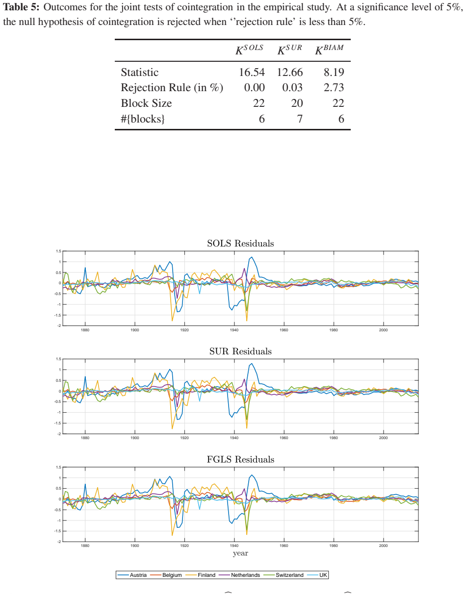
- [Section 5, Table 5] All three cointegration tests reject the null of cointegration at the 5% level, yet the paper proceeds to estimate and interpret the EKC model. The authors disclose this, but the framing should make explicit that the empirical application is illustrative and cannot serve as evidence in favor of the quadratic EKC specification, given the formal rejection.
- [References] The reference list contains two entries, Ing, Chiou, and Guo (2016a) and (2016b), with the same title and journal information. The duplication should be reconciled or the two distinct contributions should be clearly distinguished.
- [Title and Section 1] The title uses "Efficient Estimation," but the paper does not establish a formal efficiency lower bound or compare the limit distribution to a semiparametric efficiency bound. Consider qualifying the claim, for example by referring to efficiency in the GLS sense, to avoid overstating the theoretical result.
Circularity Check
No significant circularity: FM-GLS limit is derived from convergence arguments, and the sole self-citation is non-load-bearing.
full rationale
The derivation chain is self-contained against external benchmarks. Theorem 1 derives the infeasible GLS limit from the Beveridge-Nelson decomposition and standard weak convergence for cointegrating polynomial regressions; the statement that this limit coincides with Wagner et al. (2020)'s MSUR is a cross-check, not an input. Theorem 2 proves consistency of the BIAM estimator from Lemma S3 and truncation bounds, and the proof of Theorem 3(c) derives Assumption 2 from first-stage OLS rates rather than assuming it: 'Since the residuals {ˆut} are obtained by first stage OLS, we get ||ˆu−u||2 ≤ ||G−1T (ˆβOLS −β)||2 ||GT Z′ZGT || = Op(1).' The bias correction in (3.12) is constructed so that hat(B)+ estimates B+ = B_{epsilon-eta} - B_{vu}, but the mixed normal limit (3.13) follows from the convergence of each stochastic integral and the consistency of hat(B)+, not from the definition alone; this is the standard fully modified construction, not a reduction of the target to its input. The only self-citation, Beutner et al. (2019), is used as a pointer for applying the modified Cholesky block decomposition to time series; the decomposition itself is attributed to Pourahmadi (1999), Kim and Zimmerman (2012), and Kohli et al. (2016), and no theorem in the paper relies on Beutner et al. for its proof. The empirical EKC section explicitly acknowledges that the country sample was selected in Wagner et al. (2020) because it displays EKC behaviour, and the reported under-coverage of confidence intervals is a stated limitation rather than a fitted claim. No equation reduces by construction to a fitted target, and no load-bearing result is imported from a self-citation.
Assumptions & free parameters
free parameters (3)
- banding parameter q_T =
data-driven, e.g., H=[2 T^{1/4}], l0=[T/5] in Supplement S4
- block size b_T for KPSS tests =
data-driven by minimum volatility rule of Romano and Wolf
- autocovariance truncation r_T for long-run covariance estimator =
Assumption 5: r_T = O(q_T), r_T q_T^3/T -> 0
assumptions (6)
- domain assumption Assumption 1: i.i.d. innovations ζ_t with positive definite covariance, finite 2r moments, invertible VAR(∞) errors with sum j||A_j||_F < infinity.
- domain assumption Assumption 1(c): det(D(1)) != 0, so there is no cointegration among the I(1) regressors, and no cross-sectional cointegration is allowed.
- ad hoc to paper Assumption 2: first-stage OLS residuals satisfy ||\hat u - u||_2 = O_p(1).
- ad hoc to paper Assumptions 3 and 5: banding parameter q_T satisfies q_T^3/T -> 0 and r_T satisfies r_T q_T^3/T -> 0 with r_T = O(q_T).
- domain assumption Assumption 4: kernel estimators of long-run covariance matrices are consistent.
- standard math Baxter's inequality, the First Moment Bound Theorem of Findley and Wei (1993), and de Jong (2002) for nonlinear transformations of integrated processes.
Cite this review
Pith. "Pith review of Efficient Estimation by Fully Modified GLS with an Application to the Environmental Kuznets Curve." pith.science (2026). https://pith.science/paper/L3KZQEIE
@misc{pith2026190802552,
  author       = {Pith},
  title        = {Pith review of: Efficient Estimation by Fully Modified GLS with an Application to the Environmental Kuznets Curve},
  year         = {2026},
  howpublished = {\url{https://pith.science/paper/L3KZQEIE}},
  note         = {Machine review of arXiv:1908.02552}
}
read the original abstract
This paper develops the asymptotic theory of a Fully Modified Generalized Least Squares estimator for multivariate cointegrating polynomial regressions. Such regressions allow for deterministic trends, stochastic trends and integer powers of stochastic trends to enter the cointegrating relations. Our fully modified estimator incorporates: (1) the direct estimation of the inverse autocovariance matrix of the multidimensional errors, and (2) second order bias corrections. The resulting estimator has the intuitive interpretation of applying a weighted least squares objective function to filtered data series. Moreover, the required second order bias corrections are convenient byproducts of our approach and lead to standard asymptotic inference. We also study several multivariate KPSS-type of tests for the null of cointegration. A comprehensive simulation study shows good performance of the FM-GLS estimator and the related tests. As a practical illustration, we reinvestigate the Environmental Kuznets Curve (EKC) hypothesis for six early industrialized countries as in Wagner et al. (2020).
Figures
Figures from the paper (5 more)


Reference graph
Works this paper leans on
-
[1]
Abadir, K. M. and J. R. Magnus (2005). Matrix Algebra. Cambridge University Press. Anderson, T. W. and D. A. Darling (1952). Asymptotic theory o f certain “goodness of fit” criteria based on stochastic processes. The Annals of Mathematical Statistics 23 , 193–212. Andrews, D. W. K. (1991). Heteroskedasticity and autocorre lation consistent covariance matri...
work page 2005
-
[2]
follows from Lemma 1(a) and∑∞ j=q+1 j1/2 ‖ ‖ ‖A j ‖ ‖ ‖F = o(q−1/2). Using (A.2) and ‖ ‖ ‖S(q)−Σ ηη ‖ ‖ ‖→ 0 (see (S1.17) in the supplementary material), we obtain T∑ t=1 ( Aq(L)Z ′ t GT )′ S−1(q) ( Aq(L)Z ′ t GT ) = T∑ t=1 GT ZtΩ −1 uu Z ′ t GT + Op (q−1/2) ⇒ ∫ 1 0 J (r)Ω −1 uu J (r)′dr. (A.4) We rewrite the second part in (A.1) as T∑ t=1 ( Aq(L)Z ′ t GT...
work page 2016
-
[3]
for the final inequality, we derive ∑q j=1 ‖ ‖ ‖~A j(q) ‖ ‖ ‖F ≤ ∑q j=1 j ‖ ‖ ‖A j(q) ‖ ‖ ‖F ≤ ∑q j=1 j ‖ ‖ ‖A j(q) − A j ‖ ‖ ‖F +∑q j=1 j ‖ ‖ ‖A j ‖ ‖ ‖F ≤ C ∑q j=1 j ‖ ‖ ‖A j ‖ ‖ ‖F ≤ C. ■ Proof of Theorem 1 The premultiplication by Mu(q) applies a linear filter whereas S−1 u (q) im- plies weighting. Since the behaviour of the first q ≪ T elements does not...
work page 1988
-
[4]
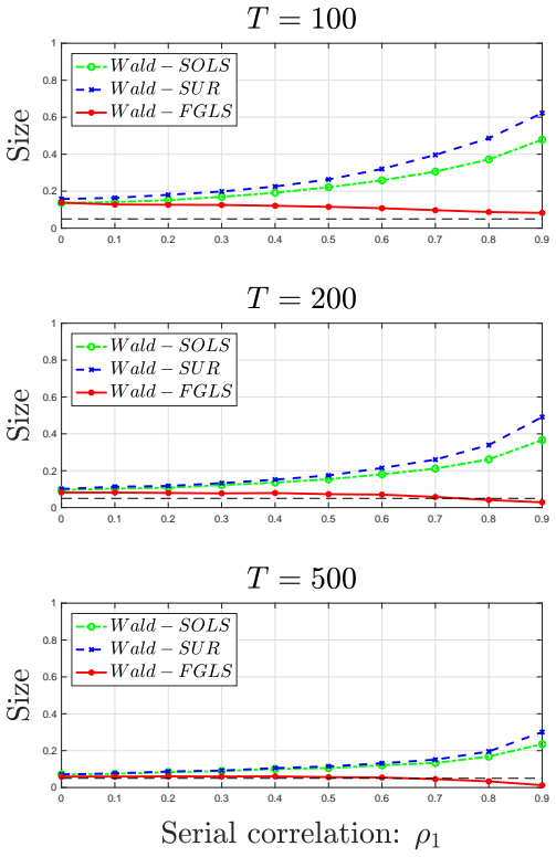
The Wald-SOLS test (green) and Wald-SUR test (blue) are bas ed on Proposition 2 by Wagner et al
n = 3 n = 5 ρ Wald-SOLS Wald-SUR Wald-FGLS Wald-SOLS Wald-SUR Wald-FGL S Panel A: Single-equation test T = 100 0 11.75 13.44 9.89 14.30 17.84 13.44 0.3 13.25 15.09 9.92 15.32 19.59 13.55 0.6 16.13 19.03 7.54 18.80 27.65 11.86 0.8 20.56 26.60 4.70 26.72 43.11 10.13 T = 200 0 9.02 10.00 7.48 9.90 12.00 8.47 0.3 9.96 10.93 7.24 11.32 13.62 8.81 0.6 12.68 14....
work page 2020
-
[7]
j] ηit ⏐ ⏐ ⏐≤ CT −3/2 ∑T t=1 |ηit| = op(1). (2) By Assumption 1, for any 1 ≤ k, i ≤ n, vkt and ηit are Near Epoch 24 Dependent in L4-norm on {[η ′ t , ε′ t]′} t∈Z of size −1 and arbitrary size, respectively. A small variation on Theorem 17.9 from Davidson (1994) shows that {vitηit} are L2-NED of size −1. The i.i.d. as- sumption on {[η ′ t , ε′ t]′}allows ...
work page 1994
-
[8]
The specific reason is as follows. By the binomial expansio n (below (A.3)), we have T −( j+1)/2 T∑ t=1 ∆x j ktηit = T −( j+1)/2 j−1∑ m=0 ( j m ) T∑ t=1 xm kt−1v j−m kt ηit = jT −( j+1)/2 T∑ t=1 x j−1 kt−1vktηit + op(1) = jΣ ǫkηi 1 T T −1∑ t=1 ( xkt √ T )j−1 + j√ T 1√ T T −1∑ t=1 ( xkt √ T )j−1 ( vktηit − Σ ǫkηi ) + op(1) ⇒ jΣ ǫkηi ∫ 1 0 B j−1 vk (r)dr, wh...
work page 2002
-
[9]
13 We conclude that ‖ ‖ ‖ˆMu(q)−Mu(q) ‖ ‖ ‖= Op (√ q3/T )
max 1≤ℓ≤q ‖ ‖ ‖ˆA(ℓ) − A(ℓ) ‖ ‖ ‖ 2 = Op (q3 T ) , where the final step follows from Lemma S3. 13 We conclude that ‖ ‖ ‖ˆMu(q)−Mu(q) ‖ ‖ ‖= Op (√ q3/T ) . The di fference ˆS −1 u (q) − S−1 u (q) forms a symmetric and block diagonal matrix, hence ‖ ‖ ‖ˆSu(q) − Su(q) ‖ ‖ ‖= max {‖ ‖ ‖ˆS(0) − S(0) ‖ ‖ ‖, max1≤ℓ≤q ‖ ‖ ‖ˆS(ℓ) − S(ℓ) ‖ ‖ ‖ } . By Assumption 2, ‖ ...
work page 2015
-
[10]
From (3.12), the definition of the FM-GLS estimator, we have G−1 T (ˆβ + FGLS − β ) = ( GT Z ′ ˆΣ −1u (q)ZG T )−1 [ GT Z ′ ˆΣ −1u (q)u − GT Z ′( IT ⊗ ˆΩ −1 uu ˆΩ uv ˆΩ −1 vv ) v − GTˆB +] . Given Theorem 2, we have GT Z ′ ˆΣ −1u (q)ZG T = GT Z ′Σ −1 u (q)ZG T + op(1) and it converges weakly to the expression in (A.4). To continue, we define ˆAq(L) = In −∑q ...
work page 2016
Show all 24 references
-
[11]
The column labeled FGLS contains the numerical value of the MSE of feasible FM-G LS
under error Setting B. The column labeled FGLS contains the numerical value of the MSE of feasible FM-G LS. Other MSEs are expressed relative to this benchmark. V alues above 1 indicate a better performance of feasible FM-GLS. n = 3 n = 5 (λ, ¯λ) T SOLS SUR FGLS infSOLS infSUR...
2020
-
[13]
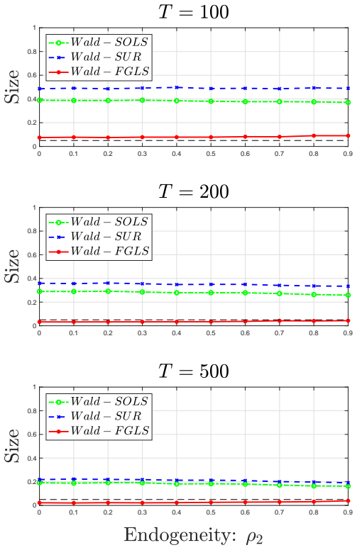
The Wald-SOLS test (green) and Wald-SUR test (blue) are bas ed on Proposition 2 by Wagner et al
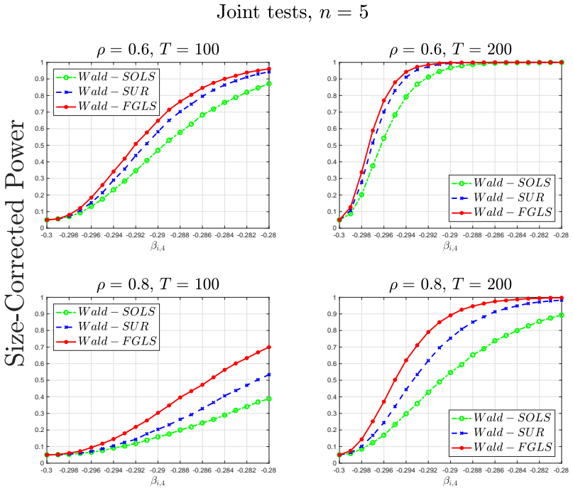
32 0 0.1 0.2 0.3 0.4 0.5 0.6 0.7 0.8 0.9 0 0.2 0.4 0.6 0.8 1 0 0.1 0.2 0.3 0.4 0.5 0.6 0.7 0.8 0.9 0 0.2 0.4 0.6 0.8 1 0 0.1 0.2 0.3 0.4 0.5 0.6 0.7 0.8 0.9 0 0.2 0.4 0.6 0.8 1 Figure 2: Empirical size of the joint Wald tests H0 : β1,4 = β2,4 = · · · = βn,4 = −0.3, where βi,4 ...
2020
-
[14]
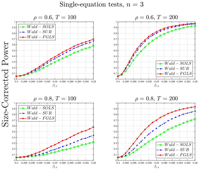
We consider n = 3, T ∈ {100, 200}, and ρ1 = ρ2 = ρ3 = ρ4 = ρ with ρ ∈ {0.6, 0.8}
33 -0.3 -0.298 -0.296 -0.294 -0.292 -0.29 -0.288 -0.286 -0.284 -0.282 -0.28 0 0.1 0.2 0.3 0.4 0.5 0.6 0.7 0.8 0.9 1 -0.3 -0.298 -0.296 -0.294 -0.292 -0.29 -0.288 -0.286 -0.284 -0.282 -0.28 0 0.1 0.2 0.3 0.4 0.5 0.6 0.7 0.8 0.9 1 -0.3 -0.298 -0.296 -0.294 -0.292 -0.29 -0.288 -0...
2020
-
[15]
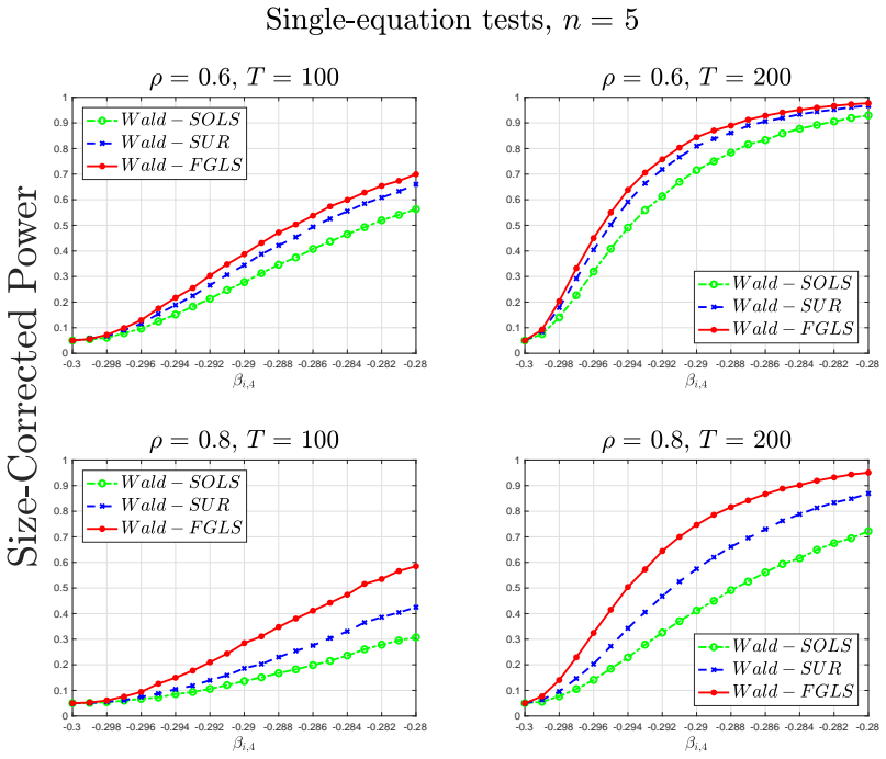
We consider n = 5, T ∈ {100, 200}, and ρ1 = ρ2 = ρ3 = ρ4 = ρ with ρ ∈ {0.6, 0.8}
34 -0.3 -0.298 -0.296 -0.294 -0.292 -0.29 -0.288 -0.286 -0.284 -0.282 -0.28 0 0.1 0.2 0.3 0.4 0.5 0.6 0.7 0.8 0.9 1 -0.3 -0.298 -0.296 -0.294 -0.292 -0.29 -0.288 -0.286 -0.284 -0.282 -0.28 0 0.1 0.2 0.3 0.4 0.5 0.6 0.7 0.8 0.9 1 -0.3 -0.298 -0.296 -0.294 -0.292 -0.29 -0.288 -0...
2020
-
[16]
We consider n = 3, T ∈ { 100, 200}, and ρ1 = ρ2 = ρ3 = ρ4 = ρ with ρ ∈ { 0.6, 0.8}
35 -0.3 -0.298 -0.296 -0.294 -0.292 -0.29 -0.288 -0.286 -0.284 -0.282 -0.28 0 0.1 0.2 0.3 0.4 0.5 0.6 0.7 0.8 0.9 1 -0.3 -0.298 -0.296 -0.294 -0.292 -0.29 -0.288 -0.286 -0.284 -0.282 -0.28 0 0.1 0.2 0.3 0.4 0.5 0.6 0.7 0.8 0.9 1 -0.3 -0.298 -0.296 -0.294 -0.292 -0.29 -0.288 -0...
2020
-
[17]
We consider n = 5, T ∈ { 100, 200}, and ρ1 = ρ2 = ρ3 = ρ4 = ρ with ρ ∈ { 0.6, 0.8}
36 -0.3 -0.298 -0.296 -0.294 -0.292 -0.29 -0.288 -0.286 -0.284 -0.282 -0.28 0 0.1 0.2 0.3 0.4 0.5 0.6 0.7 0.8 0.9 1 -0.3 -0.298 -0.296 -0.294 -0.292 -0.29 -0.288 -0.286 -0.284 -0.282 -0.28 0 0.1 0.2 0.3 0.4 0.5 0.6 0.7 0.8 0.9 1 -0.3 -0.298 -0.296 -0.294 -0.292 -0.29 -0.288 -0...
2020
-
[18]
At a significance level of 5%, the null hypothesis of cointegration is rejected when ‘’rej ection rule’ is less than 5%
38 Table 5: Outcomes for the joint tests of cointegration in the empiric al study. At a significance level of 5%, the null hypothesis of cointegration is rejected when ‘’rej ection rule’ is less than 5%. KS OLS KS UR KBIAM Statistic 16.54 12.66 8.19 Rejection Rule (in %) 0.00 0...
2012
-
[19]
We observe that ui,t = ∑∞ j=0 rowi (C j )η t− j
Recall C(L) = [A(L)]−1 = ∑∞ j=0 C jL j with C0 = In, and ∑∞ j=0 j ‖C j‖F < ∞. We observe that ui,t = ∑∞ j=0 rowi (C j )η t− j. By Proposition 10.2(b) of Hamilton (1994), abso- lute summability of the coe fficient matrices {C j}∞ j=0 implies ∑∞ s=0 |γu,k(s)| < ∞ where γu,k(s) = 4...
1994
-
[20]
Overall, this gives ‖ ‖ ‖ ‖ ‖ ‖ ‖ 1 T − q T −1∑ t=q ˆut(q)ˆut(q)′ − E(ut(q)ut(q)′) ‖ ‖ ‖ ‖ ‖ ‖ ‖= Op ( q √ T ) + Op ( q√ T ) = op(1)
Because 1 T −q ∑T −1 t=q ‖ut(q)‖= Op(q) by Markov’s inequality, we conclude Ib = Op ( q/ √ T ) . Overall, this gives ‖ ‖ ‖ ‖ ‖ ‖ ‖ 1 T − q T −1∑ t=q ˆut(q)ˆut(q)′ − E(ut(q)ut(q)′) ‖ ‖ ‖ ‖ ‖ ‖ ‖= Op ( q √ T ) + Op ( q√ T ) = op(1). (S1.11) Now observe that E(ut(q)ut(q)′)is a le...
1987
-
[21]
Collecting all the results, we have Ia ≤ C √ Kq, Ib ≤ C √ Kq, and thus ‖ ‖ ‖Fu(q) − Fu ‖ ‖ ‖1 ≤ C √ Kq
It is likewise straightforward to derive ∑T −1− j i=1 ‖Ai(i + j) − Ai(q)‖2 F ≤ CKq. Collecting all the results, we have Ia ≤ C √ Kq, Ib ≤ C √ Kq, and thus ‖ ‖ ‖Fu(q) − Fu ‖ ‖ ‖1 ≤ C √ Kq. For ‖Mu(q) − Mu‖∞, we are bounding the maximum absolute row sums. For an arbitr ary (nT ×...
1952
-
[22]
It suffices to prove ‖ ‖ ‖ˆΣ ξ(qT ) ‖ ‖ ‖= Op(1)
Finally, showing ‖ ‖ ‖ˆΣ ξ(qT )Q1 ‖ ‖ ‖= Op(1) will complete the proof after a straightforward comparison of the established stochastic orders. It suffices to prove ‖ ‖ ‖ˆΣ ξ(qT ) ‖ ‖ ‖= Op(1). Weyl’s inequality (e.g. pages 40 and 46 in Tao (2012)) an d Theorem 2 imply ⏐ ⏐ ⏐ ⏐λm...
2012
-
[23]
The BIC criterion select the V AR(1) specification for both series (Table 7)
to the series { ˆut,FGLS } and {∆xt} individually. The BIC criterion select the V AR(1) specification for both series (Table 7). St ore the coefficient matrices ˆAu and ˆAv as well as the residual series { ˆη t} and { ˆεt}, respectively. (b) Stack ˆζt = [ ˆη ′ t , ˆε′ t]′ and com...
2008
-
[24]
does not lead to qualitatively di fferent results. When we implement the minimum volatility rule as mentioned i n Section 3 to select b, the values of tuning parameters are adopted from Wagner and Hong (2016), see their online supple- mentary material. 50
2016
-
[323]
Newey, W. K. and K. D. West (1994). Automatic lag selection in covariance matrix estimation. The Review of Economic Studies 61 , 631–653. Nordhaus, W. D. (2013). The Climate Casino: Risk, Uncertainty, and Economics for a W arming World. Y ale University Press. 20 Nyblom, J. an...
1994
-
[383]
Romano, J. P . and M. Wolf (2001). Subsampling intervals in au toregressive models with linear time trend. Econometrica 69, 1283–1314. Saikkonen, P . (1992). Estimation and testing of cointegrat ed systems by an autoregressive approx- imation. Econometric Theory 8 , 1–27. Shin...
2001
-
[502]
Lin, and S
Beutner, E., Y . Lin, and S. Smeekes (2019). GLS estimation an d confidence sets for the date of a single break in models with trends. Working Paper. Bickel, P . J. and E. Levina (2008). Regularized estimation of large covariance matrices. The Annals of Statistics 36 , 199–227....
2019
Reviewed August 14, 2026 · model on record in the stance chip above.
Discussion (0). Continue with ORCID to comment.