REVIEW 2 major objections 4 minor 14 references
Finite type $\xi$-asymptotic lines of plane fields in $\mathbb{R}^3$
T0 review · 2 major / 4 minor · reviewed 2026-08-14 · deepseek-v4-flash
Pith's one-line read Any finite type curve is an asymptotic line of a suitable plane field.
desk verdict A solid local existence construction for plane-field asymptotic lines, with a real gap in Theorem 3.1 for m>2 that is probably fixable; the explicit hyperbolic closed example stands. read the letter →
The pith
A machine-rendered reading of the paper's core claim, the machinery that carries it, and where it could break.
The reading
What carries the argument
The load-bearing object is the tubular neighborhood framing $\alpha(x,y,z)=\gamma(x)+yY(x)+zZ(x)$ with $Y=(\gamma_2',-\gamma_1',0)$ and $Z=X\wedge Y$, together with the general ansatz (2.5) for a vector field $\xi$ that makes $\gamma$ an integral curve of the plane field. In these coordinates the $\xi$-asymptotic line condition becomes the implicit system $a\,dx+b\,dy+c\,dz=0$ and $L_1dx^2+\cdots+L_6dz^2=0$; when $c\neq 0$ this reduces to $dz=-(a/c)dx-(b/c)dy$ and the quadratic equation $e\,dx^2+2f\,dx\,dy+g\,dy^2=0$, whose discriminant $K=eg-f^2$ is the plane-field analogue of Gaussian curvature. The proof's engine is the factorization $b=x^{m-2}B$, $c=x^{m-2}C$ with $C(0,0,0)\neq 0$, which removes an apparent singularity at the finite type point, and the choice of the free coefficient $k_1$ forcing $K(x,0,0)=-1$. For the closed example, the same machinery feeds the linearization of the Poincaré map, $dP(0,0)=Q(l)$ from the matrix system (4.3).
What would settle it
Take the concrete finite type curve $\gamma(x)=(x,x^m,x^n)$ with $m>2$, substitute the general ansatz (2.5), impose $k_0,l_0$ from (2.6), and attempt to solve for a smooth nonzero vector field $\xi$ near the origin. If for every choice of the tail functions $A,B,C$ the coefficients after division by $x^{m-2}$ still vanish at the origin or fail to be smooth, then Theorem 3.1 fails at finite type points with $m>2$.
Extended reading notes
Core claim
The central claim is Theorem 3.1: any finite type curve $\gamma(x)=(x,a_m x^m+O_{m+1}(x),a_n x^n+O_{n+1}(x))$, with $1<m<n$ and $a_m a_n\neq 0$, is a $\xi$-asymptotic line without parabolic points of a suitable plane field. The proof places the curve in the tubular coordinates $\alpha(x,y,z)=\gamma(x)+yY(x)+zZ(x)$, where $Y=(\gamma_2',-\gamma_1',0)$ and $Z=X\wedge Y$, and writes a general vector field $\xi$ in the form (2.5). The condition that $\gamma$ is an asymptotic line fixes the low-order coefficients $k_0,l_0$ in terms of $\gamma'$ and $\gamma''$. The decisive algebraic step is that the coefficients $b(x,0,0)$ and $c(x,0,0)$ of the implicit equation share the factor $x^{m-2}$; after dividing it out, $c(0,0,0)=a_m m(m-1)\neq 0$, so the equation can be solved for $dz$, and the remaining freedom in the vector field is used to make the plane-field curvature $K=eg-f^2$ equal to $-1$ along the curve. The paper then computes, for the closed curve $\gamma(x)=(\sin x,\cos x,\sin 3x)$, the eigenvalues of $dP(0,0)$ as $e^{2\pi}$ and $e^{-25\pi/8}$, neither lying on the unit circle, proving that the closed $\xi$-asymptotic line is hyperbolic.
Load-bearing premise
In the proof of Theorem 3.1 the argument divides the common factor $x^{m-2}$ out of the coefficients of the implicit equation, and everything rests on the resulting quotient defining a smooth nonzero plane field in a neighborhood of the finite type point; if no choice of the tail functions makes that quotient smooth and nonvanishing, the construction does not produce a genuine plane field there.
Editorial extensions
If this is right
- Any finite type curve in $\mathbb{R}^3$, including curves with inflection points, can be realized as a $\xi$-asymptotic line of a plane field with no parabolic points on the curve, so the curve itself imposes no obstruction once the plane field is allowed to be non-integrable.
- Arnold's theorem for asymptotic lines on hyperbolic surfaces becomes the integrable special case of this construction; the appendix gives a new proof of that theorem through the same normal-form calculation.
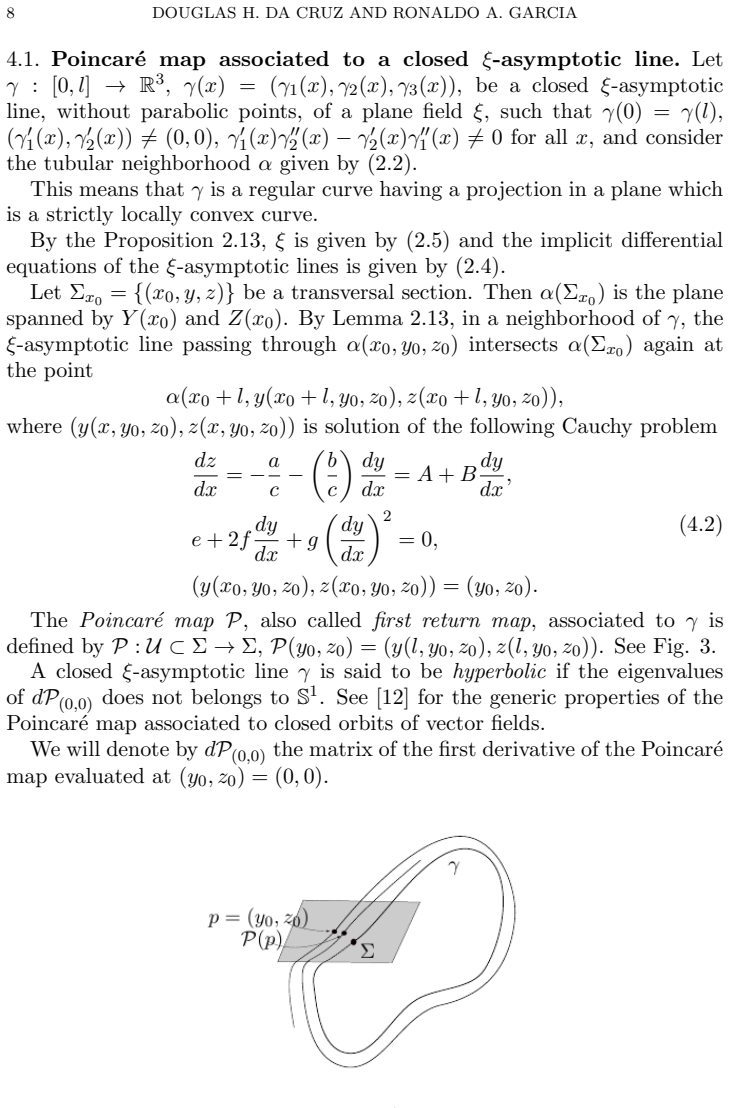
- The explicit curve $\gamma(x)=(\sin x,\cos x,\sin 3x)$ is a closed hyperbolic $\xi$-asymptotic line: the eigenvalues of its Poincaré return derivative are $e^{2\pi}$ and $e^{-25\pi/8}$, so the closed line is hyperbolic in the sense of periodic orbits.
- Because plane fields need not be integrable, closed $\xi$-asymptotic lines can have convex or starlike projections, which is impossible for closed asymptotic lines on surfaces $z=\varphi(x,y)$ by the Panov theorem quoted as Theorem 2.2; the circle example in Section 2 already exhibits this flexibility.
Reading between the lines
- The same tubular-neighborhood ansatz can likely prescribe not only the curve but also the value of the plane-field curvature along it, for instance $K=-H^2$ from Proposition 4.1, suggesting that the parabolic set of the field can be engineered to lie away from a prescribed finite type curve.
- The factorization step indicates that finite type points with $m>2$ are not singular for plane fields in the way they are for surfaces; a natural test is whether the construction extends to symbols with $m=2$ or to rotating type curves $n=m+1$ by the same division argument.
- If the theorem is true, the solution set of the implicit equation for $\xi$-asymptotic lines can be made to contain any prescribed finite type curve as a hyperbolic branch, so plane-field asymptotic foliations are substantially more flexible than surface asymptotic foliations.
- A testable extension would be the higher-dimensional analogue: whether every finite type curve in $\mathbb{R}^n$ can be realized as an asymptotic line of a suitable hyperplane field in $\mathbb{R}^n$.
Signed reviews
Editorial analysis
A structured set of objections, weighed in public.
Referee Report
Summary. The paper studies ξ-asymptotic lines of plane fields in R^3, i.e., curves whose tangent direction has zero normal curvature with respect to a plane field. The main result, Theorem 3.1, claims that every finite type curve is a ξ-asymptotic line without parabolic points of a suitable plane field. The construction uses a tubular neighborhood of the curve and an explicit vector field ξ given by (2.5), with coefficients chosen so that the Gaussian curvature K = eg - f^2 satisfies K(x,0,0) = -1. The paper also gives Theorem 4.3, an explicit closed hyperbolic finite type example γ(x) = (sin x, cos x, sin 3x), with a computation of the derivative of the Poincaré map and its eigenvalues. An appendix gives a new proof of Arnold's theorem on finite type asymptotic lines of hyperbolic surfaces.
Significance. If the main theorem is correct, it generalizes Arnold's classical results by showing that every finite type curve, including curves with inflections, can be realized as an asymptotic line (without parabolic points) of some plane field; the explicit closed hyperbolic example in Theorem 4.3 is a concrete, checkable contribution. The paper's construction is explicit and the computations for the example are detailed. However, the proof of Theorem 3.1 contains a load-bearing gap for finite type points with symbol (1,m,n), m>2, where the constructed vector field vanishes; without a repair of that gap, the main theorem is not established in full generality.
major comments (2)
- [Section 3, proof of Theorem 3.1] The step "after factoring x^{m-2} from the first equation of (2.3)" is not justified. For a finite type point with symbol (1,m,n) and m>2, equations (2.5)-(2.6) give ξ(x,0,0) = l0(x)Y(x) + k0(x)Z(x), with k0(x) = a_m m(m-1)x^{m-2} + O(x^{m-1}) and l0(x) = O(x^{n-2}), so ξ(0,0,0) = 0. The proof shows only that the restricted coefficients b(x,0,0) and c(x,0,0) factor by x^{m-2}; it does not show that the coefficient a(x,y,z) in the 1-form a dx + b dy + c dz is divisible by x^{m-2} in a neighborhood, nor that the vector field (2.5) can be rescaled by a globally defined nonvanishing function to remove the zero. Dividing the 1-form by a factor present in only two of its three coefficients requires divisibility of a as a smooth function; otherwise the operation is not defined. Without this, Proposition 2.11 and the conclusion K(x,0,0) = -1 are not established at the finite type point, so the central claim of Theorem 3.1 is not proved for m>2.
- [Section 3, formula for k1 in Theorem 3.1] The definition of k1 immediately before the final sentence of the proof divides by the factor ((γ'_1)^2 + (γ'_2)^2 + (γ'_3)^2)(γ'_1 γ''_2 - γ'_2 γ''_1). At a finite type point with symbol (1,m,n) and m>2, the second factor satisfies γ'_1(0) γ''_2(0) - γ'_2(0) γ''_1(0) = 0, so the displayed expression is singular at x=0. The proof does not specify a choice of the free function l1 that makes k1 smooth, nor does it prove that such a choice exists. Thus the constructed plane field is not shown to be smooth (or even continuous) in a neighborhood of the origin in the m>2 case. This is a second load-bearing gap in the same theorem.
minor comments (4)
- [Theorem 3.1 and Proposition 4.1] The displayed formula for k1 is typographically ambiguous: the term containing l1 does not clearly indicate its denominator. Since the proof depends on this formula, the authors should rewrite it with unambiguous parentheses and fractions.
- [Appendix A] The notation [β_u, β_v, β_uu] is used without definition; it should be defined as the mixed product (determinant) of the three vectors.
- [Definition 2.3] The definition of a finite type point requires 1 < m < n, but the subsequent sentence says that if n = m+1 then γ is of rotating type; this contradicts the strict inequality and should be rephrased, for example by saying that finite type includes the rotating case as a special limit or by separating the definitions.
- [Section 4.2] In the formula for k1 in the proof of Theorem 4.3, the denominator is a function of cos x; the authors should state explicitly that this denominator is nonvanishing for all x, since the formula otherwise could be singular on the closed curve.
Circularity Check
No circularity: the paper constructs plane fields with the stated properties rather than fitting or importing them.
full rationale
The paper's main claims are existence results. In Theorem 3.1, the vector field ξ is written in the normal form (2.5) with coefficients k0, l0 computed from the curve by (2.6), and the remaining coefficient k1 is then chosen so that K(x,0,0) = −1. This is a direct construction: the target property (γ is a ξ-asymptotic line without parabolic points) is verified from the equations after the field is built, not assumed as an input. Likewise, Proposition 4.1 specifies k1 through (4.1) with an arbitrary nonvanishing H so that K = −H^2, and Theorem 4.3 selects the free functions l1, l2, k2, k3 so that the Poincaré derivatives have the stated eigenvalues; the integrals are computed after these explicit choices. There is no fitted parameter that is later renamed as a prediction. The citations to the authors' earlier articles ([6], [7], [8]) are contextual remarks about asymptotic lines on surfaces and are not used as premises for Theorem 3.1 or Theorem 4.3. Arnold's results in [4] are used only as background and as the source of the definition of finite type curve. The reviewer's concern about the step 'after factoring x^{m-2} from the first equation of (2.3)' is a possible regularity gap for symbols with m > 2, since only the restricted coefficients b(x,0,0) and c(x,0,0) are shown to be divisible by x^{m-2}; this is a rigor issue in the proof as written, not a circular reduction, because the proof is constructing the plane field rather than deriving a conclusion from data or from an unverified self-citation.
Assumptions & free parameters
free parameters (5)
- H(x) =
1
- l1(x) =
cos x
- k3(x) =
0
- l2(x) =
determined by e_z(x,0,0) = 0
- k2(x) =
determined by e_y + 2f = 0
assumptions (3)
- standard math The implicit function theorem and standard tubular neighborhood coordinates justify reducing the asymptotic line equation to an implicit ODE.
- standard math The expression (2.5) with k0,l0 from (2.6) encodes the two conditions <xi,gamma'> = 0 and <xi,gamma''> = 0 that make gamma a xi-asymptotic line.
- ad hoc to paper At finite type points with m>2, the constructed normal vector xi is zero and the proof factors out x^{m-2}; the paper does not prove that the quotient is a smooth nonzero vector field in a neighborhood.
Cite this review
Pith. "Pith review of Finite type $\xi$-asymptotic lines of plane fields in $\mathbb{R}^3$." pith.science (2026). https://pith.science/paper/LDB2MUE2
@misc{pith2026190803253,
  author       = {Pith},
  title        = {Pith review of: Finite type $\xi$-asymptotic lines of plane fields in $\mathbbR^3$},
  year         = {2026},
  howpublished = {\url{https://pith.science/paper/LDB2MUE2}},
  note         = {Machine review of arXiv:1908.03253}
}
abstract
We prove that a finite type curve is an $\xi$-asymptotic line (without parabolic points) of a suitable plane field. It is also given an explicit example of a hyperbolic closed finite type $\xi$-asymptotic line. These results obtained here are generalizations, for plane fields, of the results of V. Arnold [4].
Figures

Figures from the paper (2 more)


Reference graph
Works this paper leans on
-
[1]
II, volume 29 of Encyclopaedia of Mathematical Sciences
Geometry. II, volume 29 of Encyclopaedia of Mathematical Sciences. Springer-Verlag, Berlin, 1993. Spaces of constant curvature, A translation of Geometriya. II, Akad. Nauk SSSR, Vsesoyuz. Inst. Nauchn. i Tekhn. Inform., Moscow, 1988, Translation by V. Minachin [V. V. Minakhin], Translation edited by `E. B. Vinberg
work page 1993
-
[2]
Y. Aminov. The geometry of vector fields . Gordon and Breach Publishers, Amster- dam, 2000
work page 2000
-
[3]
Y. Aminov. The geometry of submanifolds . Gordon and Breach Science Publishers, Amsterdam, 2001
work page 2001
-
[4]
V. I. Arnold. Topological problems in the theory of asymptotic curves. Tr. Mat. Inst. Steklova, 225(Solitony Geom. Topol. na Perekrest.):11–20, 1999
work page 1999
-
[5]
L. Euler. Recherches sur la courbure des surfaces. M´ emoires de l’Acad´ emie des Sci- ences de Berlin , 16(119–143):9, 1760
- [6]
-
[7]
R. Garcia and J. Sotomayor. Structural stability of parabolic points and periodic asymptotic lines. Mat. Contemp., 12:83–102, 1997
work page 1997
-
[8]
R. Garcia and J. Sotomayor. Differential equations of classical geometry, a qualita- tive theory. Publica¸ c˜ oes Matem´ aticas do IMPA. [IMPA Mathematical Publications]. Instituto Nacional de Matem´ atica Pura e Aplicada (IMPA), Rio de Janeiro, 2009. 12 DOUGLAS H. DA CRUZ AND RONALDO A. GARCIA
work page 2009
Show all 14 references
-
[9]
Izumiya, M
S. Izumiya, M. d. C. Romero Fuster, M. A. S. Ruas, and F. Tari. Differential geom- etry from a singularity theory viewpoint . World Scientific Publishing Co. Pte. Ltd., Hackensack, NJ, 2016
2016
-
[10]
S. G. Krantz. Convex analysis. CRC Press, 2015
2015
-
[11]
Nirenberg
L. Nirenberg. Rigidity of a class of closed surfaces. In Nonlinear Problems (Proc. Sympos., Madison, Wis., 1962) , pages 177–193. Univ. of Wisconsin Press, Madison, Wis., 1963
1962
-
[12]
Palis, Jr
J. Palis, Jr. and W. de Melo. Geometric theory of dynamical systems. Springer-Verlag, New York-Berlin, 1982. An introduction, Translated from the Portuguese by A. K. Manning
1982
-
[13]
E. R. Rozendorn. Surfaces of negative curvature. In Current problems in mathematics. Fundamental directions, Vol. 48 (Russian) , Itogi Nauki i Tekhniki, pages 98–195. Akad. Nauk SSSR, Vsesoyuz. Inst. Nauchn. i Tekhn. Inform., Moscow, 1989
1989
-
[14]
A. Voss. Geometrische Interpretation der DifferentialgleichungPdx +Qdy +Rdz = 0. Math. Ann., 16(4):556–559, 1880. Authors: Douglas H. da Cruz and Ronaldo A. Garcia Address: Instituto de Matem´ atica e Estat´ ıstica Universidade Federal de Goi´ as Campus Samambaia 74690-900 - Go...
Reviewed August 14, 2026 · model on record in the stance chip above.
Discussion (0). Continue with ORCID to comment.