REVIEW 4 major objections 4 minor 29 references
Brachistochrone on a Velodrome
T0 review · 4 major / 4 minor · reviewed 2026-08-14 · deepseek-v4-flash
Pith's one-line read Extending the brachistochrone to an active cyclist on a banked track yields a near-optimal elite descent and a final 200 m time near 9.7 s.
desk verdict A genuinely new application of brachistochrone methods to track cycling, with a plausible model and real athlete data, but the near-optimality claim outruns what is actually checked. read the letter →
The pith
A machine-rendered reading of the paper's core claim, the machinery that carries it, and where it could break.
The reading
What carries the argument
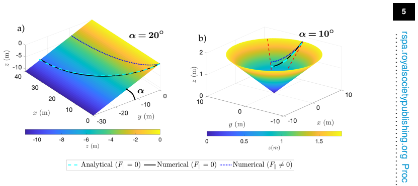
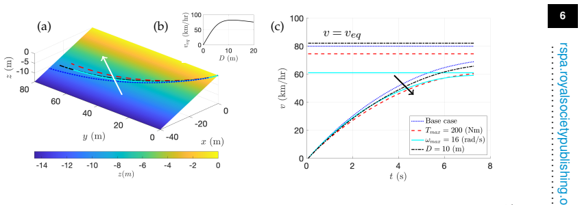
The central object is the active-particle brachistochrone: a point cyclist on a surface $z=f(x,y)$ with a pedalling force $F_\parallel$ and a perpendicular steering force $F_\perp$, so the energy changes according to $dE/dt = vF_\parallel$. The pedalling force comes from a linear torque--cadence relation $F_p = (2\pi T_{\max}/D)(1-2\pi v/(D\omega_{\max}))$, drag is quadratic $F_d=\tfrac{1}{2}\rho C_d A v^2$, and the track is encoded as $z=n\tan\alpha(s)$ with constant width $W=7.9$ m, the curved ends treated to first order in the ellipticity. The optimization discretizes the state variables in time, keeps the rider inside the track with barrier constraints, and solves the minimum-time problem with the perpendicular force as control, using a penalty and interior-point scheme; the planar and conical analytical solutions validate the numerics.
What would settle it
Recompute the same optimum on a velodrome represented with exact elliptical ends rather than the first-order expansion, and add a constraint that the normal reaction at the surface stays positive, a grip limit; if the fastest line or the final 200 m time changes by more than a few hundredths of a second, the close agreement with athlete data would be shown to be non-decisive. Alternatively, timed trials in which a rider deliberately holds a measurably different lateral line and still matches the predicted 9.7 s would indicate the model is missing a relevant constraint.
Extended reading notes
Core claim
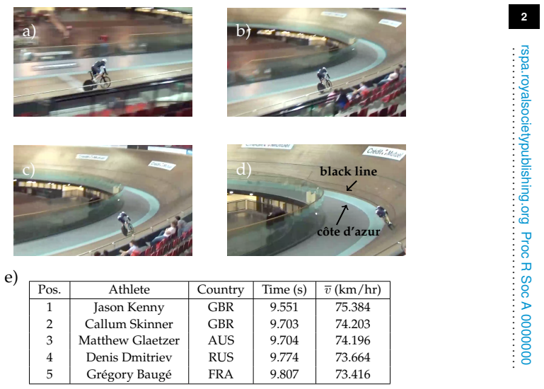
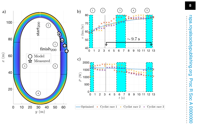
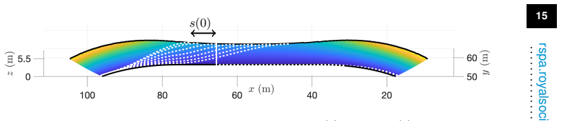
On the paper's own terms, the discovery is that the classical brachistochrone, generalized to an active particle on the measured surface of a velodrome, reproduces the elite descent closely enough to conclude that the athlete's trajectory is already nearly time-optimal. The surface is written as $z=n\tan\alpha(s)$ in tangent and normal coordinates on the track's inside lane, with the measured slope angle $\alpha(s)$ varying from about $14^\circ$ on the straights to about $45^\circ$ in the banks. Solving the time-minimization problem with pedalling torque that decreases linearly with cadence and quadratic aerodynamic drag yields an optimal line that descends before the first corner and then hugs the inside lane, with a final 200 m time near 9.7 s and velocity and power profiles that match measurements from an elite rider.
Load-bearing premise
The result depends on the measured slope, initial speed, and surface geometry being exact, on the curved ends being adequately captured by a first-order expansion in the 23% ellipticity, and on the rider being able to apply any sideways force without grip or balance limits; if any of these fails, the calculated fastest line may not be a line a real rider can hold.
Editorial extensions
If this is right
- The descent phase is the only part of a qualifying lap where rider-to-rider variation is observed, so the fractions of a second that separate medal positions come from the line chosen there; the model shows where those fractions come from.
- For a given track geometry and rider physiology, the optimal line can be computed in about 10 seconds on a laptop, making on-site tactical optimization feasible.
- The optimal start of the descent is set by the fatigue balance: peak speed should occur at the finish line, and observed starting positions from 3 m to -11 m correspond to sprint times of 13-15 s and peak speeds around 74-75 km/h.
- Riders should start from the top of the banking, because the optimal initial normal position is always $n(0)=W\cos\alpha(s(0))$, maximizing potential energy before the descent.
Reading between the lines
- One testable extension is to vary rider mass, gear development, or drag coefficient in the same solver; the model should predict how the optimal descent line and final 200 m time shift, which could be checked against athletes with different body types.
- The claim of near-optimality rests on a single rider's data on one velodrome; a stronger test would record several riders' trajectories on the same track and see whether their spread brackets the computed optimum.
- Because the curved ends are modelled only to first order in ellipticity and the steering force is unbounded, recomputing with an exact ellipse and a grip-limited normal reaction would show whether these simplifications matter at the hundredths-of-a-second level that decides races.
- If the same framework were extended to team pursuit, where slipstreaming changes the drag force, the optimal individual line might differ from the time-trial line, giving teams a quantitative tool for tactics.
Signed reviews
Editorial analysis
A structured set of objections, weighed in public.
Referee Report
Summary. The paper extends the classical brachistochrone problem to track cycling by treating a cyclist as an active point particle on a sloping surface. It first gives analytical Euler-Lagrange solutions for motion on a plane and on a cone, then solves a numerical optimal-control problem on a reconstructed model of the Montigny-le-Bretonneux velodrome. The authors compare the predicted speed and power profiles with elite-athlete measurements and conclude that the athlete's trajectory is already nearly optimal, with a final-200 m time of about 9.7 s. A separate discussion addresses the choice of initial conditions and the role of fatigue.
Significance. If the central claims hold, this is a useful and interesting contribution: it generalizes a classical variational problem to active particles on curved surfaces and provides a practical tool for optimizing track-cycling lines. The paper has clear strengths: the physiological and aerodynamic parameters are taken from independent published sources rather than fitted to the validation data; the canonical planar and conical cases provide testable analytical benchmarks; the numerical implementation is modern and reproducible in principle; and the fatigue scaling leading to Eq. (6.2) gives a simple falsifiable prediction. However, the validation claim that the athlete's trajectory is 'already nearly optimal' rests on several modeling choices that are not quantitatively checked, in particular the absence of any bound on the lateral control and the first-order treatment of the elliptical track geometry. These issues do not invalidate the overall approach, but they must be addressed before the main claim is fully supported.
major comments (4)
- [Section 3] The printed Eq. (3.2) has an integrand with denominator R0-R, which is dimensionally inconsistent with the energy equation (3.1). From (3.1), the speed satisfies v^2 = 2g sinα (R0-R), so the time functional should contain the square root of R0-R in the denominator. Since the reported Euler-Lagrange equation (3.3) appears to correspond to the corrected functional, Eq. (3.2) should be corrected, and the derivation should be checked for consistency.
- [Appendix B, Section 6a] The numerical optimization in Appendix B treats the lateral force F_perp as an unbounded control, subject only to the track-width inequalities in (A4). No bound on |F_perp|, no normal-reaction constraint, and no tyre-friction limit is imposed. Because F_perp does no work, the optimizer can in principle generate arbitrarily tight corners without affecting the longitudinal speed profile, so the computed line may be infeasible for a real cyclist. The paper should report the optimal F_perp profile and verify that the required lateral acceleration is within the grip and banking limits of the track. Without this check, the agreement in Fig. 5 does not establish that the athlete's trajectory is near-optimal.
- [Section 6a, Appendix A(c)] The reconstructed velodrome surface uses only first-order terms in the ellipticity parameter ε = a/b - 1 = 0.23, specifically Eqs. (A42) and (A47). This value is not small, and the expansion in Eq. (A41) contains terms proportional to ε^2/(r-a), which are singular as r tends to the inner boundary. The optimal trajectory is reported to hug the inside lane, so the first-order approximation may be used precisely where it is least reliable. The authors should quantify the truncation error in the optimal path and time, for example by comparing with a full-ellipse formulation or by including second-order terms.
- [Section 6b, Section 5] Fatigue is introduced only in Section 6b as a scaling argument for the initial conditions and the sprint time, Eq. (6.2). The optimal-control model that produces Fig. 5, however, uses the non-fatiguing pedalling force (5.1), with no fatigue term in the dynamics. Since the final 200 m takes about 9.7 s, longer than the stated ~5 s validity of pure anaerobic respiration, the absence of fatigue in the optimization may materially affect the predicted speed and power over the interval compared with athlete data. The authors should either include fatigue in the optimal-control dynamics or justify its neglect over this time scale before claiming full validation.
minor comments (4)
- [Section 6a] The phrase 'an an asymptotic expansion' contains a duplicated article and should read 'an asymptotic expansion'.
- [Figure 5 caption] The shaded straight regions in Fig. 5(b,c) are not defined in the caption; please state explicitly which intervals correspond to the straight sections of the track.
- [Section 5] The sentence 'In Fig. 2 we plot solutions...' appears after the physiological model is introduced, but the reader may expect the figure to be introduced near the earlier analytical discussion; consider renumbering or moving the figure reference to improve readability.
- [Section 6b] The derivation of the initial speed from a balance between constant aerobic power and drag is plausible, but the value 58 km/hr is presented without showing the numerical solution of P0/v = 1/2 ρ CdA v^2; including the intermediate calculation would make the result easier to check.
Circularity Check
Starting-height 'optimum' restates an observed input, but the main trajectory validation is independent.
-
fitted input called prediction
[Section 6(a) Validation setup and Section 6(b) Discussion of parameters and fatigue]
"For this example, we use the same parameter values as before, except with initial positions(0) = 0,n (0) =W cosα(0), and an initial velocity of 58 km/hr purely in the x-direction, which corresponds to the typical speed before descent for Olympic athletes [...] We find that the optimum value of n(0) is always given by n(0) = W cosα(s(0)), which is in accordance with our observation that track cyclists always begin their descent from the top of the velodrome ramp."
The stated 'optimum' n(0) formula is exactly the value imposed as the initial condition for the validation run: the paper sets n(0)=W cosα(0) because that is the observed top-of-ramp starting position, and then reports 'we find' the same top-of-ramp expression as optimal. Since the feasible set is 0 ≤ n ≤ W cosα and n(0) enters the dynamics only through the initial potential energy, the maximizing value is the upper bound already used as input. This is a restatement of the imposed initial condition rather than an independent prediction. It does not reduce the central claim, because the optimal trajectory and the speed/power profiles are still computed from the equations of motion rather than fitted to the measured athlete curves.
full rationale
The main derivation is self-contained against the athlete data: the equations follow from Lagrangian/Newtonian mechanics; the physiological parameters Tmax, omega_max, CdA, D, P0 and tau come from independent published sources; and the initial speed of 58 km/hr is derived from a power balance rather than tuned to the measured power/speed curves. No parameter is fitted to the elite cyclist data used for validation. The computed strategy of descending before the first corner and then hugging the inside lane is a genuine output of the optimal-control problem, not an imposed constraint, and the final-200 m time near 9.7 s is an output of the dynamics. The unbounded lateral-force control noted in Appendix B is a physical-realism or feasibility concern, not a circularity. The only mild circularity is the initial-height discussion, where an observed starting condition is presented as an optimum; this does not bear on the central near-optimality validation.
Assumptions & free parameters
free parameters (7)
- T_max =
260 Nm (from Dorel et al. [11])
- omega_max =
25 rad/s (from Dorel et al. [11])
- D =
8.5 m
- CdA =
0.22 m^2
- m =
86 kg
- Fatigue parameters P0/m, Pmax/m, tau =
6.35 W/kg, 17.4 W/kg, 38 s (from Sanders and Heijboer [25])
- Initial conditions =
s(0)=0, n(0)=W cos alpha(0), v(0)=58 km/hr
assumptions (8)
- standard math The Euler-Lagrange equations give the global minimum of the time functionals (2.3) and (3.2) under the stated boundary conditions.
- domain assumption A cyclist can be modeled as a point mass, with no rolling resistance, bike lean inertia, or steering dynamics.
- domain assumption Pedal torque is a linearly decreasing function of cadence (5.1), with T_max and omega_max from Dorel et al. [11].
- domain assumption Air drag is Fd = 1/2 rho CdA v^2 with constant CdA and no wind or drafting.
- domain assumption The velodrome surface is exactly z = n tan alpha(s) with constant width W and measured alpha(s).
- ad hoc to paper Elliptical curved sections can be represented to first order in epsilon = a/b - 1 = 0.23.
- domain assumption The lateral control F_perp is unbounded in the optimal control problem.
- ad hoc to paper The optimal strategy makes peak velocity occur exactly at the finish line, so sprint time is found by equating fatigue-limited power to drag power there.
Cite this review
Pith. "Pith review of Brachistochrone on a Velodrome." pith.science (2026). https://pith.science/paper/LM4TGFJN
@misc{pith2026190802224,
  author       = {Pith},
  title        = {Pith review of: Brachistochrone on a Velodrome},
  year         = {2026},
  howpublished = {\url{https://pith.science/paper/LM4TGFJN}},
  note         = {Machine review of arXiv:1908.02224}
}
read the original abstract
The Brachistochrone problem, which describes the curve that carries a particle under gravity in a vertical plane from one height to another in the shortest time, is one of the most famous studies in classical physics. There is a similar problem in track cycling, where a cyclist aims to find the trajectory on the curved sloping surface of a velodrome that results in the minimum lap time. In this paper we extend the classical Brachistochrone problem to find the optimum cycling trajectory in a velodrome, treating the cyclist as an active particle. Starting with two canonical cases of cycling on a sloping plane and a cone, where analytical solutions are found, we then solve the problem numerically on the reconstructed surface of the velodrome in Montigny le Bretonneux, France. Finally, we discuss the parameters of the problem and the effects of fatigue.
Figures
Figures from the paper (4 more)


Reference graph
Works this paper leans on
-
[1]
16rspa.royalsocietypublishing.org Proc R Soc A 0000000
LN Hand and JD Finch. 16rspa.royalsocietypublishing.org Proc R Soc A 0000000. . . . . . . . . . . . . . . . . . . . . . . . . . . . . . . . . . . . . . . . . . . . . . . . . . . . . . . . . . Analytical mechanics. Cambridge University Press, 1998
work page 1998
-
[2]
The brachistochrone problem and modern control theory
HJ Sussmann and JC Willems. The brachistochrone problem and modern control theory. Contemporary trends in nonlinear geometric control theory and its applications (Mexico City, 2000) , pages 113–166, 2002
work page 2000
-
[3]
A History of the Calculus of Variations from the 17th through the 19th Century , volume 5
HH Goldstine. A History of the Calculus of Variations from the 17th through the 19th Century , volume 5. Springer Science & Business Media, 2012
work page 2012
-
[4]
Brachistochrone with coulomb friction
N Ashby, WE Brittin, WF Love, and W Wyss. Brachistochrone with coulomb friction. American Journal of Physics , 43(10):902–906, 1975
work page 1975
-
[5]
On the analytical solution of the brachistochrone problem in a non-conservative field
B Vratanar and M Saje. On the analytical solution of the brachistochrone problem in a non-conservative field. International Journal of Non-Linear Mechanics , 33(3):489–505, 1998
work page 1998
-
[6]
Brachistochrone with coulomb friction
JC Hayen. Brachistochrone with coulomb friction. International Journal of Non-Linear Mechanics , 40(8):1057–1075, 2005
work page 2005
-
[7]
Time-optimal control of rolling bodies
G Perantoni and DJN Limebeer. Time-optimal control of rolling bodies. International Journal of Control , 86(11):2006–2021, 2013
work page 2006
-
[8]
The elastochrone: the descent time of a sphere on a flexible beam
JM Aristoff, C Clanet, and JWM Bush. The elastochrone: the descent time of a sphere on a flexible beam. Proceedings of the Royal Society A: Mathematical, Physical and Engineering Sciences , 465(2107):2293–2311, 2009
work page 2009
Show all 29 references
-
[9]
Time-optimal quantum evolution
A Carlini, A Hosoya, T Koike, and Y Okudaira. Time-optimal quantum evolution. Physical Review Letters, 96(6):060503, 2006
2006
-
[10]
https://assetrio2016.azureedge.net/_odf-documents/c/t/CTM001900_ Results_2016_08_12_2797f6c2_59ec_47cc_b9ba_934d32474041.pdf, 2019
Rio 2016 archives. https://assetrio2016.azureedge.net/_odf-documents/c/t/CTM001900_ Results_2016_08_12_2797f6c2_59ec_47cc_b9ba_934d32474041.pdf, 2019. Accessed: 23-07-2019
2016
-
[11]
Torque and power-velocity relationships in cycling: relevance to track sprint performance in world-class cyclists
S Dorel, CA Hautier, O Rambaud, David Rouffet, E Van Praagh, J-R Lacour, and M Bourdin. Torque and power-velocity relationships in cycling: relevance to track sprint performance in world-class cyclists. International Journal of Sports Medicine , 26(09):739–746, 2005
2005
-
[12]
The science of cycling
EW Faria, DL Parker, and IE Faria. The science of cycling. Sports Medicine, 35(4):285–312, 2005
2005
-
[13]
Mathematical physics
E Butkov. Mathematical physics. Addison Wesley Publishing Co, 1968
1968
-
[14]
Mechanics of cycling
JP Mariot. Mechanics of cycling. Revue de Physique Appliquée , 19(4):349–357, 1984
1984
-
[15]
Aerodynamic drag and biomechanical power of a track cyclist as a function of shoulder and torso angles
L Underwood, J Schumacher, J Burette-Pommay, and M Jermy. Aerodynamic drag and biomechanical power of a track cyclist as a function of shoulder and torso angles. Sports Engineering, 14(2-4):147–154, 2011
2011
-
[16]
Flow topology in the wake of a cyclist and its effect on aerodynamic drag
TN Crouch, D Burton, NAT Brown, MC Thompson, and J Sheridan. Flow topology in the wake of a cyclist and its effect on aerodynamic drag. Journal of Fluid Mechanics , 748:5–35, 2014
2014
-
[17]
Riding against the wind: a review of competition cycling aerodynamics
TN Crouch, D Burton, ZA LaBry, and KB Blair. Riding against the wind: a review of competition cycling aerodynamics. Sports Engineering, 20(2):81–110, 2017. 17rspa.royalsocietypublishing.org Proc R Soc A 0000000
2017
-
[18]
The heat of shortening and the dynamic constants of muscle
AV Hill. The heat of shortening and the dynamic constants of muscle. Proceedings of the Royal Society of London. Series B-Biological Sciences , 126(843):136–195, 1938
1938
-
[19]
Numerical optimization, second edition
J Nocedal and SJ Wright. Numerical optimization, second edition . Springer, 2006
2006
-
[20]
On the implementation of an interior-point filter line-search algorithm for large-scale nonlinear programming
A Wächter and LT Biegler. On the implementation of an interior-point filter line-search algorithm for large-scale nonlinear programming. Mathematical Programming, 106(1):25–57, 2006
2006
-
[21]
Validation of a mathematical model for road cycling power
JC Martin, DL Milliken, JE Cobb, KL McFadden, and AR Coggan. Validation of a mathematical model for road cycling power. Journal of Applied Biomechanics , 14(3):276–291, 1998
1998
-
[22]
The understanding and development of cycling aerodynamics
RA Lukes, SB Chin, and SJ Haake. The understanding and development of cycling aerodynamics. Sports Engineering, 8(2):59–74, 2005
2005
-
[23]
An experimental study on aerodynamic performance of time trial bicycle helmets
H Chowdhury and F Alam. An experimental study on aerodynamic performance of time trial bicycle helmets. Sports Engineering, 17(3):165–170, 2014
2014
-
[24]
Understanding sprint-cycling performance: the integration of muscle power, resistance, and modeling
JC Martin, CJ Davidson, and ER Pardyjak. Understanding sprint-cycling performance: the integration of muscle power, resistance, and modeling. International Journal of Sports Physiology and Performance , 2(1):5–21, 2007
2007
-
[25]
The anaerobic power reserve and its applicability in professional road cycling
D Sanders and M Heijboer. The anaerobic power reserve and its applicability in professional road cycling. Journal of Sports Sciences , 37(6):621–629, 2019
2019
-
[26]
Cyclist drag in team pursuit: influence of cyclist sequence, stature, and arm spacing
T Defraeye, B Blocken, E Koninckx, P Hespel, P Verboven, B Nicolai, and J Carmeliet. Cyclist drag in team pursuit: influence of cyclist sequence, stature, and arm spacing. Journal of Biomechanical Engineering , 136(1):011005, 2014
2014
-
[27]
Aerodynamics of human-powered vehicles
CR Kyle and MD Weaver. Aerodynamics of human-powered vehicles. Proceedings of the Institution of Mechanical Engineers, Part A: Journal of Power and Energy , 218(3):141–154, 2004
2004
-
[28]
Jump: A modeling language for mathematical optimization
I Dunning, J Huchette, and M Lubin. Jump: A modeling language for mathematical optimization. SIAM Review, 59(2):295–320, 2017
2017
-
[29]
Julia: A fresh approach to numerical computing
J Bezanson, A Edelman, S Karpinski, and VB Shah. Julia: A fresh approach to numerical computing. SIAM Review, 59(1):65–98, 2017
2017
Reviewed August 14, 2026 · model on record in the stance chip above.
Discussion (0). Continue with ORCID to comment.