Ensemble Kalman filter for multiscale inverse problems

Andrea Zanoni; Assyr Abdulle; Giacomo Garegnani

REVIEW 3 major objections 4 minor 19 references

Ensemble Kalman filter for multiscale inverse problems

T0 review · 3 major / 4 minor · reviewed 2026-08-14 · deepseek-v4-flash

Challenge this review Re-run · record.json Download PDF Read on arXiv ↗ Review JSON

Pith's one-line read This paper proves that an ensemble Kalman filter can use a cheap homogenized surrogate for oscillatory multiscale PDEs and still converge to the filter built on the exact multiscale model.

desk verdict A genuinely new combination of EnKF with homogenization, with solid conditional theorems, but the central result leans on an unverified particle-boundedness assumption that likely fails for Gaussian noise. read the letter →

arxiv 1908.05495 v2 pith:M4TAFULO submitted 2019-08-15 math.NA cs.NA

Assyr Abdulle , Giacomo Garegnani , Andrea Zanoni This is my paper · ORCID

classification math.NAcs.NA MSC 62G0565N2174Q05

keywords inverseproblemsmultiscaleellipticPDEshomogenizationensembleKalmanfilterBayesianinferencemodellingerrorFE-HMM

verification ladder T0 review T1 audit T2 compute T3 formal

The pith

A machine-rendered reading of the paper's core claim, the machinery that carries it, and where it could break.

The reading

This paper aims to establish that the ensemble Kalman filter (EnKF) for inverse problems governed by multiscale elliptic PDEs can be run with a homogenized surrogate forward map instead of the exact oscillatory solver, and still provably converge to the same result. It proves that the ensemble of recovered parameters from the surrogate-based filter converges to the ensemble from the exact multiscale filter as the oscillation scale $\varepsilon$ and the finite-element mesh size $h$ tend to zero, with the explicit rate $C(\varepsilon + h^{s+1})$. The same convergence is proved for the empirical posterior distributions in the Wasserstein distance. This matters because it turns an often computationally infeasible procedure—many solves of a finely resolved oscillatory PDE inside the filter—into a cheap coarse-mesh computation whose error is quantified and controlled.

What carries the argument

The load-bearing mechanism is a one-step error recursion, Lemma 4: if $u_n^\varepsilon$ and $u_n^0$ are the ensembles from the exact multiscale map and the exact homogenized map at iteration $n$, then $\mathbb{E}[\|u_{n+1}^\varepsilon - u_{n+1}^0\|] \le \alpha \mathbb{E}[\|u_n^\varepsilon - u_n^0\|] + \gamma \mathbb{E}[e(\varepsilon,u_n^0)]$, where $e(\varepsilon,u)$ is the mean squared forward-map difference $(1/J)\sum_j \|G^\varepsilon(u^{(j)}) - G^0(u^{(j)})\|^2$. Combining this recursion with Lemma 2 (homogenization error $\le K\varepsilon$) and Lemma 5 (finite-element error $\le \tilde K h^{s+1}$) gives the theorem. The recursion closes because Lemma 3 proves the empirical covariance matrices used in the Kalman gain are bounded and Lipschitz as functions of the ensemble, provided all particles stay in the ball of Assumption 3.

What would settle it

Take a small ensemble (say $J=10$) with a prior of unbounded support and a large Kalman gain, run the homogenized EnKF, and record the particle norms after each update: if any particle leaves $B_R(u_*)$, Assumption 3 is violated and the hypotheses of Theorem 1 are not satisfied. Alternatively, fix $\varepsilon$ and $h$, sample $E_i = G^\varepsilon(u_i) - G_h^0(u_i)$ for i.i.d. prior draws, and apply a normality test to the empirical distribution; a decisive rejection would falsify the Gaussian modelling-error model of Section 4 for that problem.

Watch

Extended reading notes

Core claim

The central discovery is Theorem 1: under Lipschitz regularity of the tensor and observation operators and an assumed bound on all particles, the ensembles produced by the EnKF with the homogenized finite-element surrogate $G_h^0$ and with the exact multiscale map $G^\varepsilon$ satisfy $\mathbb{E}[\| u_N^\varepsilon - u_{N,h}^0 \|] \le C(\varepsilon + h^{s+1})$, where $s=\min\{r,q\}$ depends on the finite-element degree and the regularity of the homogenized solution. Theorem 2 transfers this ensemble convergence to the empirical Bayesian posterior measures, which converge weakly in $L^1$ as $\varepsilon,h\to 0$. The proof separates homogenization error from discretization error and shows each is propagated linearly through the Kalman update, so the surrogate is not merely cheaper but faithful in the small-$\varepsilon$, small-$h$ limit.

Load-bearing premise

The load-bearing premise is Assumption 3: every particle of the ensemble stays, at every iteration, inside a fixed ball $B_R(u_*)$ around the true parameter; the paper gives no mechanism by which the EnKF updates would guarantee this, and without it the covariance estimates and the error recursion fail.

Editorial extensions

If this is right

Practitioners can replace each multiscale forward solve in an EnKF by a homogenized coarse-mesh solve, reducing cost by roughly the ratio of fine to coarse degrees of freedom while keeping an explicit error of order $\varepsilon + h^{s+1}$.
The Bayesian statement implies that uncertainty quantifications obtained from the cheap filter, such as credible intervals and posterior means, are consistent, as $\varepsilon,h\to 0$, with those obtained from the full multiscale model.
The modelling-error analysis gives a rule for choosing how many full multiscale solves are needed in offline estimation: $N_E = O(\eta^{-2}\log(\alpha^{-1})(\varepsilon^2 + h^{2(s+1)}))$ for the mean, and a quartic analogue for the covariance.
Because the limits in $\varepsilon$ and $h$ can be interchanged, the guarantee is insensitive to which parameter is reduced first in a convergence study.
Convergence of ensembles in the ensemble norm implies convergence of the empirical measures in the Wasserstein metric $W_{1,2}$, so point estimations and posterior distributions improve together.

Reading between the lines

Editorial extensions of the paper, not claims the author makes directly.

A direct extension of the argument would replace Assumption 3 by an algorithmic safeguard—for instance, projecting particles back into a fixed ball after each update—which would make the convergence theorem unconditional rather than conditional on the dynamics staying bounded.
The same exact-map-versus-cheap-surrogate recursion should apply to other surrogate forward maps, such as reduced-order or data-driven models, whenever the surrogate error admits a bound like Lemma 2 and the forward maps are Lipschitz; this suggests a general template for certified EnKF surrogates.
The bounds in Theorem 3 predict that the required number of full multiscale solves for modelling-error estimation shrinks quadratically (mean) or quartically (covariance) with $\varepsilon$ and $h$, a scaling one could test empirically by varying $\varepsilon$ at fixed noise level.
The posterior convergence is established for the weak Wasserstein metric; stronger distances would require additional assumptions, so the result should not be read as a total-variation or pointwise posterior guarantee.

Share X Bluesky LinkedIn Reddit HN

Signed reviews

No signed human review yet.

Editorial analysis

A structured set of objections, weighed in public.

Desk editor's note, referee report, and a circularity audit.

Desk Editor's Note

read the letter

Here's my take. The paper does something new and useful: it replaces the expensive multiscale forward solver inside an ensemble Kalman filter with a homogenized finite-element surrogate, then proves the filter error decays as ε + h^{s+1}. That's a clean, practical result. Theorems 3 and 4, which budget how many full multiscale solves are needed to estimate the modelling error, are also genuinely new and likely useful. The proofs are mostly solid; the self-citations to [2,3] set up the problem but the convergence analysis here is not circular.

The soft spots are real. The biggest is Assumption 3. All the covariance bounds and the error recursion need every particle to stay inside a fixed ball around the true parameter. The paper never shows the EnKF update preserves that ball, and with Gaussian observation noise it cannot: the update is a linear combination that includes the unbounded noise, so there is positive probability of leaving the ball in one step. The stress-test note is right. This leaves the main theorem conditional on a property the algorithm is not known to satisfy. It may be repairable—via a probabilistic radius, a bounded-noise model, or an explicit propagation estimate—but as written it is a genuine gap.

Second, Lemma 4 misstates the noise structure. The ensemble at step n depends on the fixed noise realization η from the data, so the variables ζ^(j) = η^(j)+η are not i.i.d. and not independent of the ensembles. Conditioning on η and tracking ‖η‖ would fix the computation, with slightly worse constants. Minor in the long run, but it should be corrected.

Third, the Gaussian modelling error assumption is acknowledged as heuristic; fine as an assumption, but the paper would be stronger if it offered real justification beyond a one-dimensional reference. The numerical section is illustrative: no code, a few plots, no detailed convergence check against a known truth.

Net: this deserves a serious referee. It is a solid contribution that needs a major revision to tighten the particle-boundedness argument. I would bring it to a reading group as an example of a clean conditional convergence theorem with a load-bearing but unverified assumption.

Referee Report

3 major / 4 minor

Summary. This paper proposes an ensemble Kalman filter (EnKF) method for inverse problems governed by multiscale elliptic PDEs, replacing the expensive multiscale forward map G^ε by a homogenized finite-element surrogate G^0_h obtained via FE-HMM. The main theoretical results are Theorem 1, an explicit-rate convergence of the EnKF ensemble with the surrogate to the ensemble with the exact multiscale map as ε,h→0, and Theorem 2, a corresponding L^1 weak/Wasserstein convergence of the empirical posterior measures. The paper also gives sample-size bounds for offline and online estimation of the modelling error (Theorems 3 and 4) and a numerical experiment recovering a discontinuous coefficient from boundary-flux observations.

Significance. If the convergence results hold, the paper makes a useful contribution by transferring the EnKF machinery to multiscale inverse problems with a rigorous homogenization/discretization error decomposition and explicit rates. The detailed proofs and the quantitative sample-size bounds for modelling-error estimation are strengths. However, the central theorems depend on an unverified and generically false invariant-ball assumption, and the noise handling in Lemma 4 contains a correlation error; these issues must be resolved before the main claims are reliable.

major comments (3)

[§2.3, Assumption 3; §3.1, Lemma 4] Assumption 3 is load-bearing but no mechanism is given for its propagation. In the update (16), the increment contains C_up(C_pp+Γ)^{-1} η^{(j)}_{n+1} with η^{(j)}_{n+1}∼N(0,Γ); whenever the empirical gain is non-zero, which is generic for a non-collapsed ensemble, any particle in B_R(u*) has positive probability of leaving B_R(u*) in one step, and an initial i.i.d. Gaussian ensemble is contained in B_R(u*) only with probability strictly less than one. The constants in Lemma 3 and the bound of the data-misfit factors in Lemma 4 (e.g., the use of ‖Gε(u*)−Gε(u^{(j)}_n)‖≤C_G R) all require this assumption, so Theorems 1 and 2 establish convergence only conditionally on an event that the algorithm does not guarantee. The paper should either prove a propagation result (for example by adding a projection onto B_R(u*) after each update) or reformulate the theorems as conditional on this event, ideally with a probability estimate.
[§3.1, Lemma 4] The statement in the proof of Lemma 4 that ζ^{(j)}_{n+1}=η^{(j)}_{n+1}+η are i.i.d. and independent of uε_n,u0_n is not correct for the algorithm as specified. The observation y in (8) is a single fixed vector; writing y=Gε(u*)+η introduces one realization η that is reused at every iteration n and for every particle, so the variables ζ^{(j)}_{n+1} are correlated across n and (through the history of the ensembles) dependent on uε_n and u0_n. If instead η is treated as random, the same draw is used at all iterations, so i.i.d.-ness across n still fails. This invalidates the step going from E[‖uε_n−u0_n‖(C_G R+‖ζ‖)] to α1 E[‖uε_n−u0_n‖]. The argument can likely be repaired by working with fixed y and assuming a deterministic bound on ‖y−Gε(u)‖ on B_R(u*), or by conditioning on y, but as written the proof does not go through.
[§3.2, Theorem 2] Theorem 2 inherits Assumption 3, and this is more than a technicality here: the Wasserstein distance W_{1,2} in Lemma 6 is computed on the metric space (B_R(u*),‖·‖_2), so the empirical measures μ^ε and μ^0_h must be supported in B_R(u*). Since the paper does not show that particles remain in this ball, the Bayesian convergence statement is again conditional on the unproved event of Assumption 3. In addition, the notation '{μ^ε−μ^0_h} L1 ⇀ 0' is informal because the difference of two probability measures is not a probability measure and the mode of convergence in Definition 1 is defined for random measures; the proof actually establishes E[W_{1,2}(μ^ε,μ^0_h)]→0, which should be the stated conclusion.

minor comments (4)

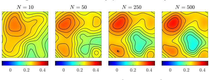
[§5.1–§5.2] The numerical setup is inconsistent: §5.1 fixes ε=1/64 for the data, while §5.2 reports experiments with ε=1/32 and with varying ε. Please clarify whether the true observations are recomputed for each value of ε in Figures 4–6.
[§4] The Gaussian modelling-error assumption E(u)∼N(m,Σ) with m and Σ independent of u is explicitly acknowledged to lack theoretical justification; this should be presented as a modelling assumption whose validity is heuristic, and the text should state that Theorems 1–2 do not depend on it.
[§1, §3, §4] There are several typos and grammatical slips: 'a inverse problems' in the introduction, 'if this work' in Section 3, and 'witch' instead of 'which' in the proof of Theorem 4. A careful proofread is needed.
[Appendix, Lemma 7] The final step of Lemma 7 ('extend to all bounded continuous functions by density') is terse; since Lipschitz functions are dense in the sup norm on the compact space B_R(u*), one sentence of justification would make the argument self-contained.

Circularity Check

0 steps flagged · score 0.0 of 10

No significant circularity: the convergence proof decomposes into external homogenization and FEM estimates, an independent EnKF stability argument, and an explicit (if unverified) boundedness assumption.

full rationale

The paper's central claims are conditional convergence results comparing the EnKF run with the homogenized FE-HMM forward map to the EnKF run with the exact multiscale map. The derivation chain does not reduce to its own inputs. Lemma 4 (the one-step recursion) is an adaptation of the independent EnKF stability framework of Iglesias-Law-Stuart and Schillings-Stuart, which are external references [11,17]. The two error terms that drive the recursion are handled by Lemma 2, whose rate E <= K eps uses the external homogenization result [12] (Moskow-Vogelius), and Lemma 5, whose rate is the standard finite-element a priori estimate cited to [7,9]. Neither term is fitted from the EnKF output, and neither is renamed as a prediction. The self-citations [2,3] are used to frame the multiscale inverse-problem setting and to motivate the modelling-error correction in Section 4, but the new convergence proof does not lean on those papers for its key inequalities. Assumption 3, requiring all particles to remain in a fixed ball B_R(u*), is a genuine conditional assumption: the paper does not prove the EnKF update preserves this ball, and with Gaussian noise this is a nontrivial limitation. However, an unproved or possibly false assumption is a correctness/robustness concern, not a circularity, because the theorem is stated conditionally on it rather than assuming the desired convergence. Similarly, the Gaussian modelling-error assumption in Section 4 is explicitly acknowledged to lack theoretical justification and is used only for the modelling-error estimation section, not for Theorems 1-2. No fitted parameter is called a prediction, no uniqueness theorem is imported from the authors, and no ansatz is smuggled in via self-citation. The numerical experiments compare against data generated from the exact multiscale model and therefore provide an external check rather than a restatement of the assumptions.

Assumptions & free parameters 0 free parameters · 7 assumptions · 0 invented entities

The central proofs rely on standard homogenization and FEM estimates plus three explicit assumptions. The only ad hoc assumptions are Assumption 3 (bounded particles) and the Gaussian modelling error model. No new physical entities are introduced.

assumptions (7)

domain assumption Assumption 1: the tensor A_u is uniformly elliptic and Lipschitz in u.
Used throughout to obtain Lipschitz continuity of the forward map (Lemma 1) and to validate the numerical example (Section 5.1).
domain assumption Assumption 2: the observation operator O is Lipschitz from H^1_0(Ω) to Y.
Required in Lemma 2 and Lemma 5 to translate solution error into observation error.
ad hoc to paper Assumption 3: all particles remain in a fixed ball B_R(u*) at every iteration.
Needed for the boundedness and Lipschitz constants in Lemma 3 and for the error recursion in Lemma 4. No mechanism guarantees this property; it is a strong algorithmic assumption.
standard math Standard periodic homogenization theory: existence of A^0_u and L^2 convergence p^ε → p^0 with rate O(ε) when p^0 ∈ H^2.
Used in Lemma 2 to obtain e(ε,u) → 0 and the rate Kε, citing [8,12].
standard math Standard finite element a priori error estimates for elliptic problems.
Used in Lemma 5 to obtain the O(h^(s+1)) bound, citing [7,9].
standard math The Bayesian interpretation of the EnKF with scaled gain from Schillings and Stuart [17].
Basis of Theorem 2 that the empirical measure of the ensemble approximates the posterior; treated as external background result.
ad hoc to paper The modelling error E(u) = G^ε(u) - G^0_h(u) is Gaussian with mean m and covariance Σ independent of u.
The paper states 'There is no theoretical guarantee for the modelling error to be distributed as a Gaussian in this framework'; the assumption is justified only by a one-dimensional study [13].

how reviews work

0 comments

Cite this review

Pith. "Pith review of Ensemble Kalman filter for multiscale inverse problems." pith.science (2026). https://pith.science/paper/M4TAFULO

@misc{pith2026190805495,
  author       = {Pith},
  title        = {Pith review of: Ensemble Kalman filter for multiscale inverse problems},
  year         = {2026},
  howpublished = {\url{https://pith.science/paper/M4TAFULO}},
  note         = {Machine review of arXiv:1908.05495}
}

read the original abstract

We present a novel algorithm based on the ensemble Kalman filter to solve inverse problems involving multiscale elliptic partial differential equations. Our method is based on numerical homogenization and finite element discretization and allows to recover a highly oscillatory tensor from measurements of the multiscale solution in a computationally inexpensive manner. The properties of the approximate solution are analysed with respect to the multiscale and discretization parameters, and a convergence result is shown to hold. A reinterpretation of the solution from a Bayesian perspective is provided, and convergence of the approximate conditional posterior distribution is proved with respect to the Wasserstein distance. A numerical experiment validates our methodology, with a particular emphasis on modelling error and computational cost.

Figures

Figures reproduced from arXiv: 1908.05495 by the authors.

**Figure 2.** EnKF estimation after N = {10, 50, 250, 500} iterations. Moreover, since the EnKF algorithm estimates the coefficients {um}M m=1 of the truncated KarhunenLoève expansion, we show that Aε (u): RM → L∞(Ω, R d×d ), which maps u into Aε σu , is Lipschitz. In fact we first have kA ε (u1) − A ε (u2)kL∞(Ω,Rd×d) ≤ √ 13e σ + sup x∈Ω |σu1 (x) − σu2 (x)| , then using the truncated Karhunen-Loève expansion and the Cauchy-Schwa… view at source ↗

**Figure 3.** EnKF estimation after N = 500 iterations with ensemble size J = {10, 100, 500, 1000} [PITH_FULL_IMAGE:figures/full_fig_p022_3.png] view at source ↗

Figures from the paper (3 more)

**Figure 4.** Figure 4: EnKF estimation after N = 500 iterations for the multiscale parameter ε = {1/4, 1/8, 1/16, 1/32}. approximation becomes worse when ε is bigger, indeed the homogenized problem becomes too different with respect to the multiscale one and, if ε is too big, the solution do…

**Figure 5.** Figure 5: EnKF with offline modeling error estimation after 500 iterations for the multiscale parameter ε = {1/4, 1/8, 1/16, 1/32} [PITH_FULL_IMAGE:figures/full_fig_p023_5.png]

**Figure 6.** Figure 6: EnKF with online iterative modeling error estimation after 500 iterations for the multiscale parameter ε = {1/4, 1/8, 1/16, 1/32}. on the ensemble originating from our multiscale algorithm converges to the measure generated by the true model, again as ε and h go to zer…

Discussion (0). Continue with ORCID to comment.

Reference graph

Works this paper leans on

19 extracted references · 18 canonical work pages

[1]

Abdulle, A priori and a posteriori error analysis for numerical homogenization: a uniﬁed framework, Ser

A. Abdulle, A priori and a posteriori error analysis for numerical homogenization: a uniﬁed framework, Ser. Contemp. Appl. Math. CAM, 16 (2011), pp. 280–305

work page 2011
[2]

Abdulle and A

A. Abdulle and A. Di Blasio , Numerical homogenization and model order reduction for multiscale inverse problems, Multiscale Model. Simul., 17 (2019), pp. 399–433

work page 2019
[3]

Uncertain

, A Bayesian Numerical Homogenization Method for Elliptic Multiscale Inverse Problems, SIAM/ASA J. Uncertain. Quantif., 8 (2020), pp. 414–450

work page 2020
[4]

Abdulle, W

A. Abdulle, W. E, B. Engquist, and E. V anden-Eijnden , The heterogeneous multiscale method, Acta Numer., 21 (2012), pp. 1–87

2012
[5]

Calvetti, M

D. Calvetti, M. Dunlop, E. Somersalo, and A. Stuart , Iterative updating of model error for Bayesian inversion, Inverse Problems, 34 (2018), pp. 025008, 38

work page 2018
[6]

Calvetti, O

D. Calvetti, O. Ernst, and E. Somersalo , Dynamic updating of numerical model discrepancy using sequential sampling, Inverse Problems, 30 (2014), pp. 114019, 19

work page 2014
[7]

P. G. Ciarlet , The ﬁnite element method for elliptic problems., vol. 40 of Classics Appl. Math., SIAM, Philadelphia, 2002

work page 2002
[8]

Cioranescu and P

D. Cioranescu and P. Donato , An introduction to homogenization, vol. 17 of Oxford Lecture Series in Mathematics and its Applications, Oxford University Press, New York, 1999

work page 1999

Show all 19 references

[9]

L. C. Evans , Partial diﬀerential equations, vol. 19 of Graduate Studies in Mathematics, American Mathematical Society, Providence, RI, second ed., 2010

2010
[10]

Evensen , Sequential data assimilation with a nonlinear quasi-geostrophic model using Monte Carlo methods to forecast error statistics, J

G. Evensen , Sequential data assimilation with a nonlinear quasi-geostrophic model using Monte Carlo methods to forecast error statistics, J. Geophys. Res., (1994), pp. 10143–10162

1994
[11]

M. A. Iglesias, K. J. H. Law, and A. M. Stuart , Ensemble Kalman methods for inverse problems, Inverse Problems, 29 (2013), pp. 045001, 20

2013
[12]

Moskow and M

S. Moskow and M. Vogelius , First-order corrections to the homogenised eigenvalues of a periodic composite medium. a convergence proof, Proc. Roy. Soc. Edinburgh, 127A (1997), pp. 1263–1299

1997
[13]

Nolen and G

J. Nolen and G. Papanicolaou , Fine scale uncertainty in parameter estimation for elliptic equations, Inverse Problems, 25 (2009), pp. 115021, 22

2009
[14]

Nolen, G

J. Nolen, G. A. Pavliotis, and A. M. Stuart , Multiscale modeling and inverse problems, in Numerical analysis of multiscale problems, vol. 83 of Lect. Notes Comput. Sci. Eng., Springer, Heidelberg, 2012, pp. 1–34

2012
[15]

Salsa, Partial diﬀerential equations in action, vol

S. Salsa, Partial diﬀerential equations in action, vol. 99 of Unitext, Springer, [Cham], third ed.,
[16]

Santambrogio, Optimal transport for applied mathematicians, vol

F. Santambrogio, Optimal transport for applied mathematicians, vol. 87 of Progress in Nonlinear Diﬀerential Equations and their Applications, Birkhäuser/Springer, Cham, 2015. Calculus of variations, PDEs, and modeling

2015
[17]

Schillings and A

C. Schillings and A. M. Stuart , Analysis of the ensemble Kalman ﬁlter for inverse problems, SIAM J. Numer. Anal., 55 (2017), pp. 1264–1290

2017
[18]

A. M. Stuart, Inverse problems: a Bayesian perspective, Acta Numer., 19 (2010), pp. 451–559. 27

2010
[2016]

From modelling to theory, La Matematica per il 3+2

Pith tools

Reviewed August 14, 2026 · model on record in the stance chip above.

[1] [1]

Abdulle, A priori and a posteriori error analysis for numerical homogenization: a uniﬁed framework, Ser

A. Abdulle, A priori and a posteriori error analysis for numerical homogenization: a uniﬁed framework, Ser. Contemp. Appl. Math. CAM, 16 (2011), pp. 280–305

work page 2011

[2] [2]

Abdulle and A

A. Abdulle and A. Di Blasio , Numerical homogenization and model order reduction for multiscale inverse problems, Multiscale Model. Simul., 17 (2019), pp. 399–433

work page 2019

[3] [3]

Uncertain

, A Bayesian Numerical Homogenization Method for Elliptic Multiscale Inverse Problems, SIAM/ASA J. Uncertain. Quantif., 8 (2020), pp. 414–450

work page 2020

[4] [4]

Abdulle, W

A. Abdulle, W. E, B. Engquist, and E. V anden-Eijnden , The heterogeneous multiscale method, Acta Numer., 21 (2012), pp. 1–87

2012

[5] [5]

Calvetti, M

D. Calvetti, M. Dunlop, E. Somersalo, and A. Stuart , Iterative updating of model error for Bayesian inversion, Inverse Problems, 34 (2018), pp. 025008, 38

work page 2018

[6] [6]

Calvetti, O

D. Calvetti, O. Ernst, and E. Somersalo , Dynamic updating of numerical model discrepancy using sequential sampling, Inverse Problems, 30 (2014), pp. 114019, 19

work page 2014

[7] [7]

P. G. Ciarlet , The ﬁnite element method for elliptic problems., vol. 40 of Classics Appl. Math., SIAM, Philadelphia, 2002

work page 2002

[8] [8]

Cioranescu and P

D. Cioranescu and P. Donato , An introduction to homogenization, vol. 17 of Oxford Lecture Series in Mathematics and its Applications, Oxford University Press, New York, 1999

work page 1999