REVIEW 4 major objections 5 minor 1 cited by
Dynamics and Control of Additional Food Provided Prey-Predator Systems exhibiting Holling Type-III Functional Response and Intra-specific Competition among Predators
T0 review · 4 major / 5 minor · reviewed 2026-08-16 · deepseek-v4-flash
Pith's one-line read The paper claims that adding food to predators in a Holling type-III prey-predator model with predator competition creates bistability, hysteresis, and bang-bang time-optimal control schedules.
desk verdict A systematic ODE analysis of a new predator-prey model, undermined by a control section that solves the wrong objective. read the letter →
The pith
A machine-rendered reading of the paper's core claim, the machinery that carries it, and where it could break.
The reading
What carries the argument
The argument runs on the model (3) with the Holling type-III denominators $1+x^2+\alpha\xi$, the quadratic predator crowding term $-\epsilon y^2$, the nullcline equations, the quintic equilibrium equation determining $x^*$, and the time reparameterization $dt=(1+\alpha\xi+x^2)\,ds$. The reparameterization is the load-bearing device for the control claims: it makes the control appear linearly in the Hamiltonian, turning the search for minimum time into a linear problem whose optimum is bang-bang or singular.
What would settle it
For the parameter values and endpoint states of the simulations in Section 9.3, take the reported optimal trajectory, compute the actual elapsed time $T=\int_0^S (1+\alpha\xi+x^2(s))\,ds$, and solve the same rendezvous by minimizing $T$ directly; if the reported trajectory's $T$ exceeds the directly minimized $T$, the time-optimality claim is refuted.
Extended reading notes
Core claim
The paper claims that system (3), which couples logistic prey growth to a Holling type-III predation term and to predators that receive additional food and compete among themselves, has a complete qualitative theory: solutions stay positive and bounded; up to five interior equilibria can occur; stability is governed by $x^{*2} < 1+\alpha\xi$; the system undergoes transcritical and saddle-node bifurcations as the quantity of additional food $\xi$ varies, and Hopf bifurcation as predator crowding $\epsilon$ varies; the interior-equilibrium curve is S-shaped, producing two saddle-node folds and a hysteresis loop under a slow periodic sweep of $\epsilon$; and in the $(\alpha,\xi)$ plane the dynamics split into regions of no interior equilibrium, unique stable interior equilibrium, or bistability between the predator-free and interior equilibria. For pest management, the paper argues the pest-free equilibrium is always saddle when it exists, so eradication is unstable, and pest population can be held to a low-pest branch by slow releases; the minimum stable pest density is $\frac{\epsilon}{1+\epsilon/\gamma}$. For control, it formulates two minimum-time problems and claims the change of independent variable $dt=(1+\alpha\xi+x^2)\,ds$ converts them into control-linear problems whose optimal policies are bang-bang or singular.
Load-bearing premise
The shortest-time conclusion depends on the assumption that replacing the real clock $t$ by the new variable $s$ through $dt=(1+\alpha\xi+x^2)\,ds$ leaves the meaning of "minimum time" intact; since $T=\int_0^S (1+\alpha\xi+x^2)\,ds$, minimizing $S$ is not generally the same as minimizing $T$.
Editorial extensions
If this is right
- Pest eradication is not a stable outcome: whenever the predator-only equilibrium exists, it is a saddle, so the operational goal must be a low-pest interior equilibrium.
- The S-shaped equilibrium curve plus two folds means slow changes in predator crowding produce hysteresis: the system stays on one branch past the fold and then jumps, so release history, not just release amount, decides which pest level is reached.
- The minimum stable pest population is set by predator crowding as $\frac{\epsilon}{1+\epsilon/\gamma}$; below that floor the interior equilibrium cannot be pushed, so competition strength determines how low pest density can go.
- In the $(\alpha,\xi)$ plane, additional food divides the dynamics into regions with no interior equilibrium, a unique stable interior equilibrium, and bistability between predator-free and interior states, so the effect of food supplementation depends on initial populations.
- The optimal control problems with quality or quantity of additional food as control are reduced, according to the paper, to linear-in-control problems, so the optimal strategies are bang-bang with possible singular arcs.
Reading between the lines
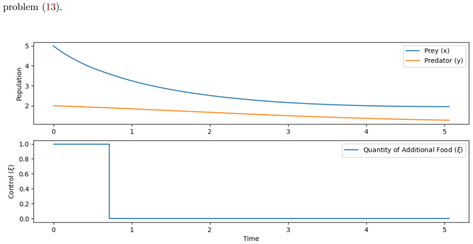
- From the equations as written, problems (13) and (19) minimize $S$, not the actual elapsed time $T$, because the reparameterization factor $1+\alpha\xi+x^2$ is state-dependent; the reported optimal times of 2.1 and 5.05 units may be values of $S$, so the schedules may not be time-optimal for the original system.
- A repair is available in principle: minimize $\int_0^S (1+\alpha\xi+x^2)\,ds$ over the same linearized dynamics, or derive the maximum-principle conditions in the original time variable; the switching curves in the paper would change under either correction.
- The hysteresis structure suggests a testable management protocol: ramp natural-enemy additions slowly to hold the low-pest branch, and avoid pulse releases large enough to cross the second fold into a high-pest jump.
Signed reviews
Editorial analysis
A structured set of objections, weighed in public.
Referee Report
Summary. The paper analyzes a two-species prey–predator model with Holling type-III functional response, additional food supplied to predators, and intra-specific competition among predators. After nondimensionalization, the authors prove positivity and attempt to prove boundedness and global existence of solutions, classify equilibria and their local stability, and derive transcritical, saddle-node, and Hopf bifurcation results. They also present numerical evidence of a hysteresis loop, study the global dynamics in the α–ξ parameter plane, and formulate time-optimal control problems in which the quality or the quantity of additional food is the control. The control problems are treated by introducing a new time variable via dt = (1 + αξ + x²) ds, which the authors claim converts each time-optimal problem into a linear problem for the pseudo-time S; bang-bang and singular control conditions are derived and simulated with CasADi for pest-management scenarios.
Significance. The model and the intended application to biological pest control are topical, and the paper contains a fairly complete nullcline-based stability classification as well as an explicit numerical demonstration of hysteresis. The control section is the most distinctive contribution, and the authors are transparent that this is an initial attempt. However, the central claims are not reliable as written: the boundedness proof is invalid, the saddle-node bifurcation theorem violates the stated Sotomayor condition, and the time-rescaling in the control sections changes the objective so that the Pontryagin analysis and simulations solve a pseudo-time problem rather than the advertised minimum-time problem. Because the latter error is load-bearing for the main novelty, the results cannot be accepted in their present form.
major comments (4)
- [Section 3.2, Theorem 3.1] The boundedness proof uses an invalid inequality. After the displayed computation, the authors bound the right-hand side by γ(1+K)²/4 + ξ/ε + (K−m)²/(4ε), but the y-dependent terms ξy/(1+x²+αξ) + ((K−m)/δ)y − (ε/δ)y² cannot be bounded in this way. Even using ξy/(1+x²+αξ) ≤ ξy, the maximum over y is δ(ξ + (K−m)/δ)²/(4ε), not ξ/ε + (K−m)²/(4ε); the factor δ is missing and the numerator of the quadratic term is not handled. A concrete counterexample to the displayed bound is obtained with α=0, m=0, K=0, x=0, ξ=10, ε=1, δ=1, and y=5, where the left-hand side is 25 while the proposed bound is γ/4+10, which is smaller for γ<60. Since this bound is the only argument for ultimate boundedness and hence for global existence of the solution, Theorem 3.1 is not proved as stated. The argument may be repairable, but the present proof is not valid.
- [Section 6.2, Theorem 6.2] The saddle-node bifurcation claim fails the authors' own Sotomayor condition. In the proof, they assert that WᵀH_ξ(E₂;ξ*) = δ(δξ−m(1+αξ))/(ε(1+αξ)³) ≠ 0. But at the stated bifurcation value ξ* = m/(δ−mα), the factor δξ−m(1+αξ) is exactly zero, so this quantity is zero, not nonzero. Thus the Sotomayor nondegeneracy condition required for a saddle-node bifurcation is not satisfied. Moreover, at this parameter value E₂ coincides with E₀=(0,0), and the exchange between these equilibria has the character of a transcritical bifurcation rather than a saddle-node bifurcation. The theorem, and the numerical discussion of Figure 3 that refers to it, therefore do not establish the claimed bifurcation.
- [Section 9.1, Eqs. (12)–(13)] The transformation dt = (1+αξ+x²)ds does not preserve the time-optimal objective. The original problem (12) minimizes T = ∫₀ᵀ dt. Under the change of variable, this becomes T = ∫₀^S (1+αξ(s)+x(s)²)ds, and since α is the control and x varies along the trajectory, the integrand is not constant. The linear problem (13) minimizes only S, dropping the factor 1+αξ+x² from the cost. Hence a control that is optimal for (13) need not be time-optimal for (12): a trajectory with smaller pseudo-time S can have a larger actual time T if it keeps 1+αξ+x² large. Consequently, the Hamiltonian, the adjoint equations, the switching conditions (14)–(17), and the singular-arc analysis characterize the pseudo-time problem, not the stated minimum-time problem. This is a load-bearing error for the paper's main pest-management application.
- [Sections 9.2–9.3] The same objective error affects the quantity-control problem: Eq. (19) minimizes S after the same transformation, but the actual time in problem (18) is still ∫₀^S (1+αξ+x²)ds. The numerical simulations in Section 9.3 solve (13) and (19) and then report the resulting 'optimal time' values (2.1 and 5.05 units), but those numbers are the pseudo-time S, not the physical time T. The control trajectories and pest-management conclusions in Figures 11 and 12 are therefore not supported as solutions of the time-optimal problems (12) and (18).
minor comments (5)
- [Throughout] There are several typographical errors, including 'Hysterisis' in the Section 6.4 heading and the abstract, 'guarentees' in Section 3.2, and 'atmost' in Section 4. The manuscript would benefit from a careful proofreading pass.
- [MSC codes] The MSC codes 60H10, 60J65, and 60J70 are stochastic-analysis codes and appear irrelevant to this deterministic dynamical-systems paper; the authors should replace them with appropriate codes such as 34C23, 92D25, and 49J15.
- [Section 5.1, Eq. (10)] In the displayed simplification of the determinant, the variables x and y are used without explicitly indicating that the expression is evaluated at (x*, y*); this makes the formula hard to follow.
- [Section 9.3] The control bounds α_min, α_max, ξ_min, and ξ_max are never specified, and the simulation section does not state the values of the bounds or the discretization parameters used in the CasADi multiple-shooting implementation, which limits reproducibility.
- [Section 7] The division of the α–ξ parameter space into regions is presented through representative phase portraits and verbal descriptions, but no theorem establishes that the listed curves exhaust the possible dynamics; this should be stated more cautiously.
Circularity Check
No significant circularity; the control and dynamics results are derived from the model equations rather than fitted or defined into existence.
full rationale
The paper's dynamical-system results (positivity, boundedness, equilibria, stability, bifurcations, hysteresis) are derived from system (3) by direct computation, with no fitted parameter renamed as a prediction. The model in (2) uses functional responses from the authors' prior work [3], but that citation supplies the modeling ansatz, not the target conclusions; the subsequent stability and control analyses do not reduce to [3]. The Section 9 transformation dt=(1+αξ+x²)ds into (13)/(19) is mathematically questionable, since minimizing S does not in general minimize T: T=∫_0^T dt=∫_0^S (1+αξ+x²) ds, so the true time cost is not constant along trajectories. However, this is a correctness/equivalence error, not circularity: the paper does not define S in terms of T, nor fit a parameter to T, nor smuggle in the conclusion via a self-citation. The 'minimum pest population ϵ/(1+ϵ/γ)' is a restatement of the lower bound in Lemma 4.1 and Theorem 5.4, which follow from the equilibrium equations and stability conditions, not from a fitted input. No load-bearing step reduces by construction to its own inputs, so the circularity score is 0.
Assumptions & free parameters
assumptions (6)
- domain assumption The biological feasibility constraint δ > m is assumed.
- ad hoc to paper The inequality γ(1+K)²/4 + ξ/ε + (K−m)²/(4ε) is an upper bound for the RHS of dW/dt + KW.
- ad hoc to paper The transformation dt = (1+αξ+x²)ds preserves the time-optimal objective.
- standard math Sotomayor's theorem applies.
- standard math Gronwall's inequality applies.
- domain assumption The additional food functional response from [3] is adopted.
Cite this review
Pith. "Pith review of Dynamics and Control of Additional Food Provided Prey-Predator Systems exhibiting Holling Type-III Functional Response and Intra-specific Competition among Predators." pith.science (2026). https://pith.science/paper/MDMT34EB
@misc{pith2026250418035,
  author       = {Pith},
  title        = {Pith review of: Dynamics and Control of Additional Food Provided Prey-Predator Systems exhibiting Holling Type-III Functional Response and Intra-specific Competition among Predators},
  year         = {2026},
  howpublished = {\url{https://pith.science/paper/MDMT34EB}},
  note         = {Machine review of arXiv:2504.18035}
}
read the original abstract
The dynamics of predator-prey systems influenced by intra-specific competition and additional food resources have increasingly become a subject of rigorous study in the realm of mathematical biology. In this study, we consider an additional food provided prey-predator model exhibiting Holling type-III functional response and the intra-specific competition among predators. We prove the existence and uniqueness of global positive solutions for the proposed model. We study the existence and stability of equilibrium points and further explore the possible bifurcations. We numerically depict the presence of Hysteresis loop in the system. We further study the global dynamics of the system and discuss the consequences of providing additional food. Later, we do the time-optimal control studies with respect to the quality and quantity of additional food as control variables by transforming the independent variable in the control system. We show that the findings of these dynamics and control studies emphasises the role of additional food and intra-specific competition in bio-control of pests.
Figures


Figures from the paper (9 more)


Forward citations
Cited by 1 Pith paper
-
Additional Food Enhances the Bifurcation Structure of Predator Competition Models
An additional-food predator-prey model with generalized predator competition is claimed to exhibit a cusp-type Bogdanov–Takens bifurcation of codimension 4 and a focus-type one of codimension 3, with up to three limit...
Reference graph
Works this paper leans on
-
[1]
Success stories in biological control: Lessons learnt,
C. R. Ballal, “Success stories in biological control: Lessons learnt,” Vantage: Journal of Thematic Analysis, vol. 3, no. 1, pp. 7–20, 2022
work page 2022
-
[2]
B. Chhetri, D. S. S. M. Kanumoori, and D. K. K. Vamsi, “Influence of gestation delay and the role of additional food in holling type III predator–prey systems: A qualitative and quantitative investigation,” Modeling Earth Systems and Environment, vol. 7, no. 2, pp. 897–915, Jun. 2021, issn: 2363-6203, 2363-
work page 2021
-
[3]
P. D. N. Srinivasu, D. K. K. Vamsi, and V. S. Ananth, “Additional food supplements as a tool for biological conservation of predator-prey systems involving type III functional response: A qualitative and quantitative investigation,” Journal of Theoretical Biology, vol. 455, pp. 303–318, Oct. 2018, issn: 00225193. doi: 10.1016/j.jtbi.2018.07.019
-
[4]
D. K. K. Vamsi, D. S. S. M. Kanumoori, and B. Chhetri, “Additional Food Supplements as a Tool for Biological Conservation of Biosystems in the Presence of Inhibitory Effect of the Prey,” Acta Biotheoretica, vol. 68, no. 3, pp. 321–355, Sep. 2020,issn: 0001-5342, 1572-8358. doi: 10.1007/s10441- 019-09371-x
-
[5]
P. D. N. Srinivasu, D. K. K. Vamsi, and I. Aditya, “Biological Conservation of Living Systems by Providing Additional Food Supplements in the Presence of Inhibitory Effect: A Theoretical Study Using Predator–Prey Models,” Differential Equations and Dynamical Systems , vol. 26, no. 1-3, pp. 213–246, Jan. 2018, issn: 0971-3514, 0974-6870. doi: 10.1007/s1259...
-
[6]
Structural and dynamic stability of model predator-prey systems,
A. Bazykin, “Structural and dynamic stability of model predator-prey systems,” 1976
work page 1976
-
[7]
Bifurcations and hydra effects in bazykin’s predator–prey model,
P. D. Adhikary, S. Mukherjee, and B. Ghosh, “Bifurcations and hydra effects in bazykin’s predator–prey model,” Theoretical Population Biology, vol. 140, pp. 44–53, Aug. 2021, issn: 10960325. doi: 10.1016/ j.tpb.2021.05.002
work page 2021
-
[8]
R. Howard, “The gronwall inequality,” lecture notes, 1998. 30
work page 1998
Show all 12 references
-
[9]
Perko, Differential equations and dynamical systems
L. Perko, Differential equations and dynamical systems . Springer Science and Business Media, 2013, vol. 7
2013
-
[10]
Cesari, Optimization—theory and applications: problems with ordinary differential equations
L. Cesari, Optimization—theory and applications: problems with ordinary differential equations. Springer Science and Business Media, 2012, vol. 17
2012
-
[11]
CasADi – A software framework for nonlinear optimization and optimal control,
J. A. E. Andersson, J. Gillis, G. Horn, J. B. Rawlings, and M. Diehl, “CasADi – A software framework for nonlinear optimization and optimal control,” Mathematical Programming Computation , vol. 11, no. 1, pp. 1–36, 2019. doi: 10.1007/s12532-018-0139-4 . 31
2019 doi
-
[6211]
doi: 10.1007/s40808-020-01042-y
Reviewed August 16, 2026 · model on record in the stance chip above.
Discussion (0). Continue with ORCID to comment.