REVIEW 3 major objections 5 minor 1 cited by
Optimal Estimation of Generalized Average Treatment Effects using Kernel Optimal Matching
T0 review · 3 major / 5 minor · reviewed 2026-08-14 · deepseek-v4-flash
Pith's one-line read The paper unifies every weighted average treatment effect estimand under a single definition and proves that Kernel Optimal Matching weights minimize worst-case error and estimate any such effect at the root-n rate.
desk verdict The fixed-V generalization of KOM is worth refereeing, but the new KOWATE/KOSATE estimand has a load-bearing normalization bug: V is constrained to sum to 1 while GATE in (2.1) and every fixed estimand use V summing to n, so the variable-V consistency claim does not follow as stated. read the letter →
The pith
A machine-rendered reading of the paper's core claim, the machinery that carries it, and where it could break.
The reading
What carries the argument
The central machinery—an RKHS-expressible worst-case bias functional that turns covariate balancing into a convex-quadratic program—is the worst-case conditional mean squared error functional $C(W_{1:n}, V_{1:n}, \lambda_{0:1})$, built from moment-discrepancy terms $\Delta_t(W_{1:n}, V_{1:n})$ measured as reproducing kernel Hilbert space (RKHS) norms. For kernels $K_0, K_1$, Theorem 3.2 gives $\Delta_t^2(W,V) = \frac{1}{n^2}\big(W^{\top} I_S I_t K_t I_t I_S W - 2 V^{\top} K_t I_t I_S W + V^{\top} K_t V\big)$, which turns bias control into a linearly constrained convex-quadratic program in the weights. Adding $\lambda$-weighted variance penalties makes the objective an estimated worst-case CMSE, and the consistency proof shows any solution of this program is no worse than normalized inverse probability weighting in CMSE, hence root-n consistent.
What would settle it
In the Section 4 simulation, compute KOM weights once with kernel hyperparameters tuned on the observed outcomes and once with hyperparameters tuned on an independent holdout split; if the resulting GATE estimates differ by more than the robust standard error, outcome leakage through tuning is material and the honesty assumption underpinning the theoretical claims is violated.
Extended reading notes
Core claim
The paper's central discovery is that the conditional mean squared error of any weighted comparison estimator decomposes into a squared bias term, measuring the discrepancy between the weighted treated and control groups relative to the V-weighted target sample in the conditional outcome functions, plus a variance term. When this discrepancy is measured by a reproducing kernel Hilbert space norm with a positive semidefinite kernel, its worst case over all functions in the unit ball becomes an exactly computable convex-quadratic function of the weights. Minimizing this worst-case CMSE over nonnegative weights that respect the treatment-group sums yields, for any fixed target estimand V, weights with the optimal bias-variance trade-off, and the resulting estimator is consistent at rate O_p(1/√n) under the paper's assumptions. When V is left free within a polytope, the same optimization simultaneously selects the estimand—the kernel optimal weighted average treatment effect—that is easiest to estimate. The paper demonstrates by simulation that this beats IPW, truncated IPW, overlap weights, and outcome regression under misspecification and positivity violations, and applies the method to spine surgery and HIV peer-support data.
Load-bearing premise
The load-bearing premise is Assumption 2.5 (honest weights)—that the weights are chosen without seeing outcomes—but Section 3.6 tunes kernel hyperparameters on the observed outcomes, so the implemented weights depend on Y and the claimed unbiasedness and CMSE decomposition do not hold exactly.
Editorial extensions
If this is right
- Any of SATE, TATE, SATT, OWATE, and OSATE can be estimated by the same code with a different fixed target weight vector V, and all enjoy the same root-n consistency guarantee.
- The KOWATE estimand, chosen by the solver, is by construction the weighted average effect with the smallest worst-case CMSE among allowed target weights, so it is the honest target when covariate overlap is limited.
- The method removes the need to estimate propensity scores for weighting: bias control comes from the kernel discrepancy, so misspecification of the propensity model no longer drives bias.
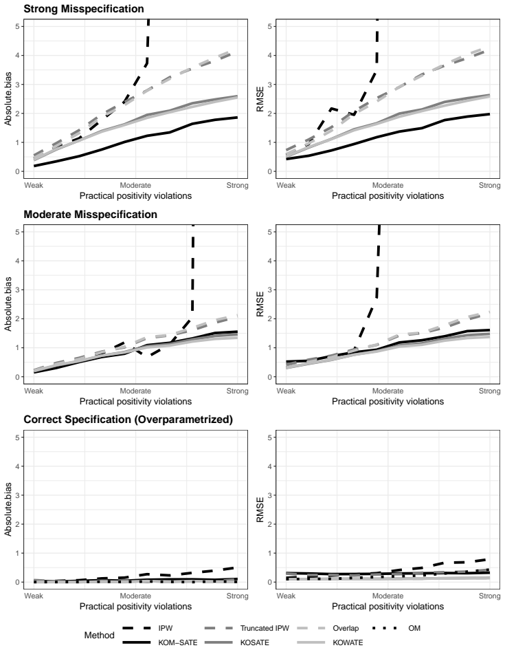
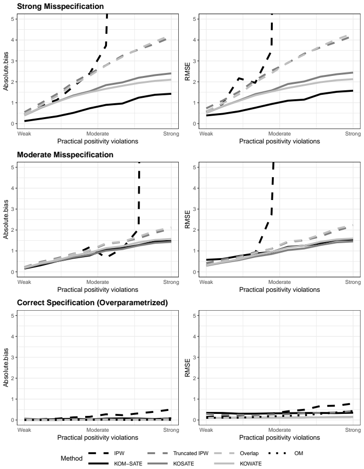
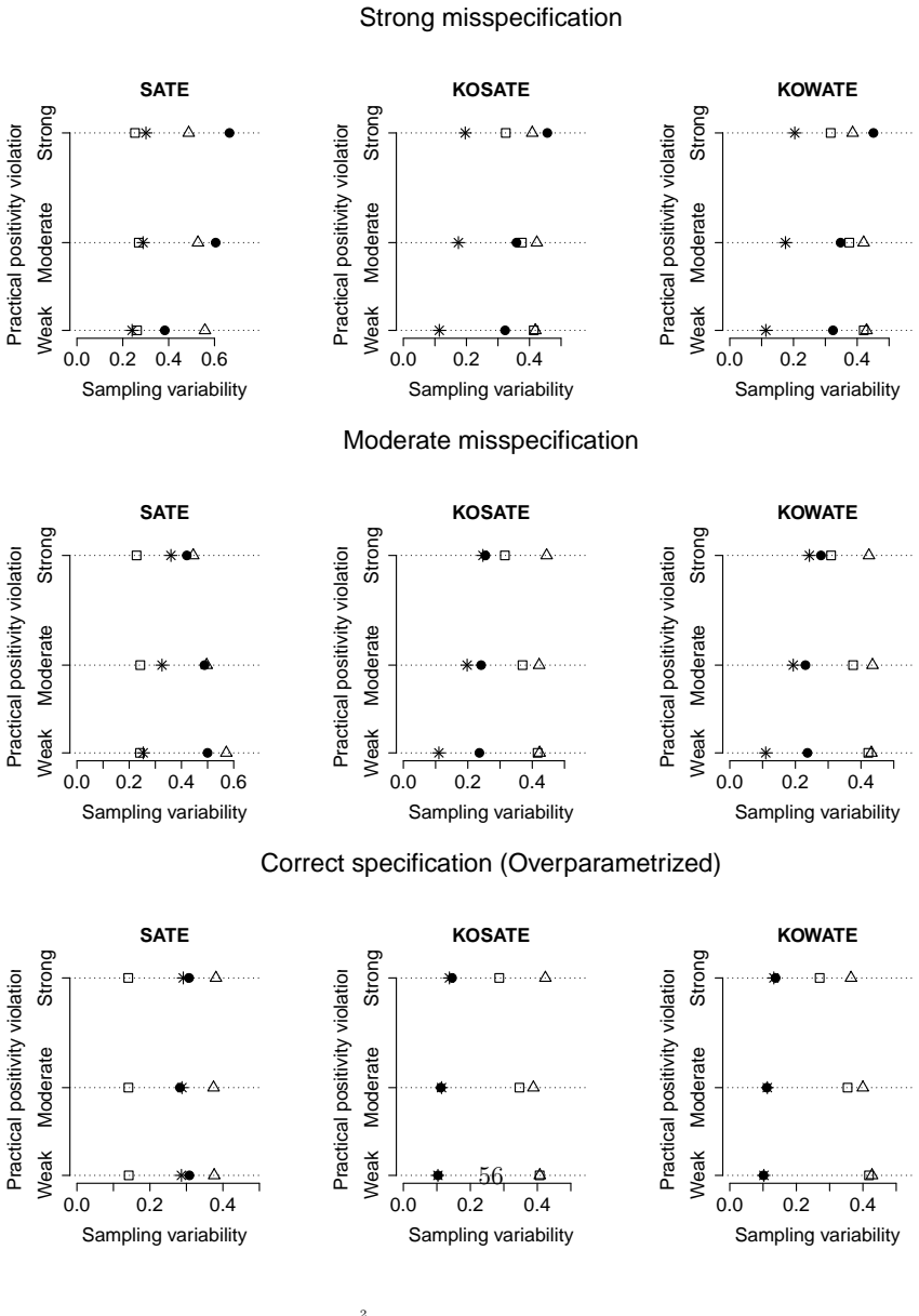
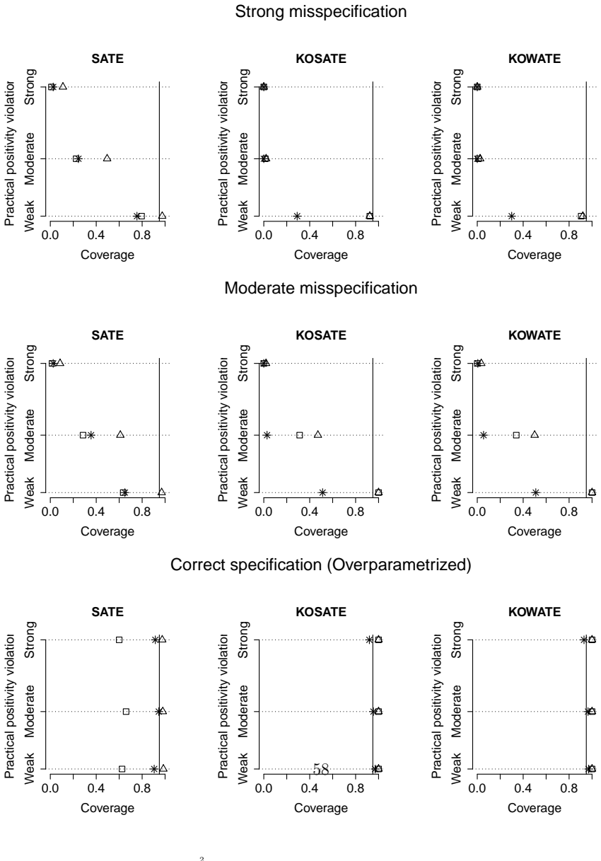
- Under strong practical positivity violation, the simulations show KOM retains low bias and RMSE where IPW and outcome regression diverge sharply.
- The method extends trial results to target populations via the TATE special case, as illustrated in the HIV peer-support analysis with healthier target populations.
Reading between the lines
- The same convex-quadratic program could be wrapped in a cross-validation loop that selects the target set V by out-of-sample CMSE, yielding a data-driven choice of estimand rather than a single KOWATE.
- Because Section 3.6 tunes kernel hyperparameters on the observed outcomes, the implemented weights violate the honest-weights assumption; a fully honest variant would tune on a separate split or use permutation calibration, and the CMSE bound would need re-derivation for adaptive weights.
- The KOSATE restriction to {0, 1/n'} suggests a direct comparison with cardinality matching on the same objective, which the paper does not pursue.
- Domain knowledge about which covariate transformations are likely misspecified could be encoded directly in the kernel choice; the paper uses a generic polynomial Mahalanobis kernel instead.
Signed reviews
Editorial analysis
A structured set of objections, weighed in public.
Referee Report
Summary. The paper proposes a unifying estimand, the Generalized Average Treatment Effect (GATE), and applies Kernel Optimal Matching (KOM) to estimate it. The GATE formulation embeds SATE, SATT, TATE, OWATE, OSATE, and other estimands as special choices of weights V. The KOM procedure minimizes a worst-case CMSE expressed as a convex quadratic program over weights, with a variance penalty, and the paper introduces KOWATE and KOSATE as estimands whose target weights are themselves chosen by the same optimization. The authors prove unbiasedness of generalized IPW weights, derive the CMSE decomposition, give consistency rates for fixed V, and illustrate the method in simulations and in two case studies. The manuscript includes detailed proofs in the supplementary material and an accompanying R implementation.
Significance. If the claims were fully established, the paper would make a useful contribution: it offers a clean unification of many causal estimands, a practical convex-quadratic formulation that can be solved with off-the-shelf software, and a coherent treatment of the fixed-V case. The fixed-V results, in particular, appear sound under the stated assumptions, and the open-source R package is a concrete strength. However, the central new estimands KOWATE and KOSATE suffer from a normalization inconsistency that breaks the stated consistency theorem, and the implemented hyperparameter tuning violates the paper's own honesty assumption. These issues are load-bearing for the paper's main novelty, so the manuscript needs substantial revision before the central claims can be accepted.
major comments (3)
- [Sections 3.3.2, 3.5, and Supplement 10.4] The KOWATE normalization is inconsistent with GATE. In Section 2, GATE is defined as tau_V = (1/n) sum_i V_i (g_1(X_i) - g_0(X_i)), and every estimand in Table 1 has sum_i V_i = n. In contrast, Section 3.3.2 restricts variable V to the simplex {V >= 0 : sum_i V_i = 1}, and Section 3.5 applies Theorem 3.3 to this choice. This cannot be correct: the feasible set W imposes sum_{i in T} W_i = sum_{i in C} W_i = n, so for a constant function g_t = c the discrepancy B_t is (1/n)(sum_{i in T} W_i - sum_i V_i) c = (n-1)c/n, which does not vanish as n grows. Concretely, with n = 2, one treated and one control unit, X_1 = X_2, g_0 = 0, and g_1 = delta, every feasible W has W_1 = W_2 = 2 and every feasible V has V_1 + V_2 = 1, so tau_V = delta/2 but the estimator equals delta, giving a fixed bias of delta/2. The proof in Supplement 10.4 makes the incompatible assumptions that E[Z_t^IPW] = 1, which requires sum_i V_i = n, and simultaneously that sum_i V_i = 1 to bound sqrt(sum_i V_i^2). The variable-V consistency claim in Theorem 3.3 is therefore not proved and is false as stated. The same scale problem affects KOSATE, which Table 2 defines with sum_i V_i = 1 while Section 5.1.2 uses sum_i V_i = n_T.
- [Section 3.6 and Assumptions 2.5, Theorem 3.3] The implemented tuning procedure invalidates the honesty assumption. Section 3.6 tunes the kernel hyperparameters theta_t and gamma_t and the noise variance sigma_t^2 by maximizing the Gaussian-process marginal likelihood of the observed outcomes, and then solves (3.5) or (3.7) with the resulting kernel. Because K_t enters the objective, the optimal W* and V* become functions of the outcome Y. Assumption 2.5 requires W and V to be independent of potential outcomes given H = {X, T, S}, and the claim in Section 3.5 that V* from (3.7) is honest because it is a function of H is therefore false for the procedure actually implemented. The unbiasedness and CMSE decomposition in Lemma 2.1 and Theorem 3.1 rely on Assumption 2.5, and Theorem 3.3 treats the kernel as fixed in its proof. Consequently, the theoretical guarantees do not cover the algorithm used in the simulations and case studies. The paper should either use sample splitting for hyperparameter tuning, or extend the theory to data-dependent kernels under explicit additional conditions, or clearly state that the implemented procedure is an approximation whose guarantees are not yet established.
- [Section 4.1] The simulation definition of the true GATE drops the 1/n from equation (2.1). The text states that the true GATE was computed as tau_V = sum_i V_i (Y_i(1) - Y_i(0)). For SATE with V_i = 1, this is n times the estimand in (2.1); for KOWATE with sum_i V_i = 1, it is also n times the estimand in (2.1), since (1/n) sum_i V_i (g_1 - g_0) is the actual target. The estimator in (2.2) contains the 1/n factor, and its weights sum to n within each treatment group, so the reported bias and RMSE numbers in Figure 2 compare quantities whose scales are not consistent across estimands. The authors should state the exact formula used in the simulations and recompute the evaluation under a single, consistently normalized definition of the estimand.
minor comments (5)
- [Section 5.1.2] The KOSATE feasible set is written as {V in {0,1} : sum_i V_i = n_T}, which conflicts with Table 2, where KOSATE is defined as {V in {0,1/n'} : sum_i V_i = 1}; please reconcile these definitions and clarify the intended normalization.
- [Section 2] There is a typo in the text introducing Lemma 2.1: 'genalized IPW weights' should read 'generalized IPW weights'.
- [Supplement 10.4] The proof of Theorem 3.3 asserts that E[W_i^{nIPW}] = 1 without justification; this is exactly the scale assumption that fails for the simplex V, as discussed in the first major comment.
- [Figure 2] The legend and the text disagree on how outcome regression modeling is plotted: the text describes it as dotted-black, while the caption lists it as dashed-light-grey; please align the description.
- [Theorem 3.3] Theorem 3.3 states assumptions 2.1-2.4 but its proof invokes the generalized IPW construction of Lemma 2.1, whose unbiasedness requires Assumption 2.5; the theorem statement should either include Assumption 2.5 or explain why it is unnecessary for the proof.
Circularity Check
Minimax KOM core is self-contained; the KOWATE 'easiest-to-estimate' claim is definitional rather than derived, and other noted issues are correctness risks, not circularity.
-
self definitional
[Section 3.3.2 and Section 3.4 (Eqs. 3.7-3.8)]
"The solution to the optimization problem (3.8) provides both weights V∗ 1:n that define a GATE of interest and the weights W∗1:n to estimate it. The weights V1:n are chosen in order to allow for minimal CMSE. That is, it focuses on the subpopulation where the average effect on which is easiest to estimate by KOM."
KOWATE is defined as the V* that minimizes the same worst-case CMSE objective C(W,V) used to define the estimator, so the property that KOWATE is 'the GATE most easily estimable by KOM' is a restatement of the optimization problem (3.7), not a theorem derived from separate overlap or estimability conditions. Any feasible V attaining the minimum of C is by construction the easiest estimand under this criterion; no independent characterization is proved. The conceptual conclusion in Section 3.4 therefore repackages the definition as a finding.
full rationale
The paper's core minimax derivation is not circular: Theorem 3.1 decomposes the CMSE, Theorem 3.2 evaluates the worst-case discrepancy in an RKHS, and the convex-quadratic programs (3.5)-(3.8) minimize that objective. For fixed V, the optimality of W* is by construction of the objective, but consistency (Theorem 3.3) is a substantive claim with a proof that does not reduce to the inputs. The use of Lemma 31 of Kallus (2016) is a final technical self-citation but concerns a standard CMSE-to-rate argument and is not an unverified premise. The main definitional circularity is KOWATE itself: its advertised property of being the most easily estimable GATE is exactly what the optimization (3.7) defines, so presenting it as an insight is a labeling move. Two additional concerns raised by the text are correctness risks rather than circularity: (i) Section 3.6 tunes kernel hyperparameters and noise variances on observed outcomes, which violates Assumption 2.5 that W and V be independent of outcomes given H, so the unbiasedness/CMSE decomposition is not exact for the implemented procedure; (ii) KOWATE's feasible set sums V_i to 1 while GATE (2.1) and every fixed estimand in Table 1 use V summing to n, and Section 4.1 computes 'true GATE' as an unnormalized sum, suggesting a scale mismatch that would invalidate the variable-V consistency claim as stated. These are serious validity concerns, but they are not cases of a prediction being equivalent to its inputs by construction, so they do not raise the circularity score above 3.
Assumptions & free parameters
free parameters (3)
- Kernel hyperparameters theta_t and gamma_t =
Tuned by GP marginal likelihood on outcomes
- Kernel polynomial degree d =
d>=2 recommended; d=2 used in simulations with fallback to d=3
- Penalization parameter lambda_t =
sigma_t^2 / gamma_t^2 estimated from GPML
assumptions (8)
- domain assumption Consistency and non-interference (SUTVA): observed outcome equals the potential outcome of the assigned treatment, and units' outcomes do not depend on others' treatment.
- domain assumption Ignorable treatment assignment (Assumption 2.1): Y_i(t) independent of T_i given X_i, S_i=1.
- domain assumption Ignorable sampling (Assumption 2.2): Y_i(t) independent of S_i given X_i.
- domain assumption Bounded propensity and sampling probabilities (Assumptions 2.3, 2.4).
- domain assumption Honest weights (Assumption 2.5): W and V independent of outcomes given H.
- domain assumption The conditional outcome functions g_t have finite RKHS norm under the chosen kernel, or a universal kernel is used with a vanishing approximation term.
- standard math PSD kernels and representer theorem for RKHS.
- domain assumption Bounded kernels and finite second moments E[K_t(X,X)] < infinity, E[V_i^2] < infinity.
invented entities (3)
-
GATE (Generalized Average Treatment Effect)
-
KOWATE (Kernel Optimal Weighted Average Treatment Effect)
-
KOSATE (Kernel Optimal Sample Average Treatment Effect)
Cite this review
Pith. "Pith review of Optimal Estimation of Generalized Average Treatment Effects using Kernel Optimal Matching." pith.science (2026). https://pith.science/paper/MMLFCIOG
@misc{pith2026190804748,
  author       = {Pith},
  title        = {Pith review of: Optimal Estimation of Generalized Average Treatment Effects using Kernel Optimal Matching},
  year         = {2026},
  howpublished = {\url{https://pith.science/paper/MMLFCIOG}},
  note         = {Machine review of arXiv:1908.04748}
}
read the original abstract
In causal inference, a variety of causal effect estimands have been studied, including the sample, uncensored, target, conditional, optimal subpopulation, and optimal weighted average treatment effects. Ad-hoc methods have been developed for each estimand based on inverse probability weighting (IPW) and on outcome regression modeling, but these may be sensitive to model misspecification, practical violations of positivity, or both. The contribution of this paper is twofold. First, we formulate the generalized average treatment effect (GATE) to unify these causal estimands as well as their IPW estimates. Second, we develop a method based on Kernel Optimal Matching (KOM) to optimally estimate GATE and to find the GATE most easily estimable by KOM, which we term the Kernel Optimal Weighted Average Treatment Effect. KOM provides uniform control on the conditional mean squared error of a weighted estimator over a class of models while simultaneously controlling for precision. We study its theoretical properties and evaluate its comparative performance in a simulation study. We illustrate the use of KOM for GATE estimation in two case studies: comparing spine surgical interventions and studying the effect of peer support on people living with HIV.
Figures


Figures from the paper (9 more)




Forward citations
Cited by 1 Pith paper
-
Target-Weighted Neyman Allocation: Experimental Design for Heterogeneous Treatment Effects under Population Shift
For target-weighted group average treatment effects under population shift, the optimal two-stage design allocates groups in proportion to sqrt(deployment share) times the sum of arm standard deviations, with the Neym...
Reference graph
Works this paper leans on
-
[1]
Buchanan, A. L., M. G. Hudgens, S. R. Cole, K. R. Mollan, P. E. Sax, E. S. Daar, A. A. Adimora, J. J. Eron, and M. J. Mugavero (2018). Generalizing evidence from randomized trials using inverse probability of sampling weights. Journal of the Royal Statistical Society: Series A (Statistics in Society)\/ 181\/ (4), 1193--1209
work page 2018
-
[2]
Cai, T., L. Tian, P. H. Wong, and L. Wei (2010). Analysis of randomized comparative clinical trial data for personalized treatment selections. Biostatistics\/ 12\/ (2), 270--282
work page 2010
-
[3]
Cain, L. E. and S. R. Cole (2009). Inverse probability-of-censoring weights for the correction of time-varying noncompliance in the effect of randomized highly active antiretroviral therapy on incident aids or death. Statistics in medicine\/ 28\/ (12), 1725--1738
work page 2009
-
[4]
Carey, T. S. (1999). Randomized controlled trials in surgery: an essential component of scientific progress. Spine\/ 24\/ (23), 2553
work page 1999
-
[5]
Cole, S. R. and M. A. Hern \'a n (2008). Constructing inverse probability weights for marginal structural models. American journal of epidemiology\/ 168\/ (6), 656--664
work page 2008
-
[6]
Cole, S. R. and E. A. Stuart (2010). Generalizing evidence from randomized clinical trials to target populations: The actg 320 trial. American journal of epidemiology\/ 172\/ (1), 107--115
work page 2010
-
[7]
Crump, R. K., V. J. Hotz, G. W. Imbens, and O. A. Mitnik (2008). Nonparametric tests for treatment effect heterogeneity. The Review of Economics and Statistics\/ 90\/ (3), 389--405
work page 2008
-
[8]
Crump, R. K., V. J. Hotz, G. W. Imbens, and O. A. Mitnik (2009). Dealing with limited overlap in estimation of average treatment effects. Biometrika\/ 96\/ (1), 187--199
2009
Show all 65 references
-
[9]
Eck, J. C., A. Sharan, Z. Ghogawala, D. K. Resnick, W. C. Watters III, P. V. Mummaneni, A. T. Dailey, T. F. Choudhri, M. W. Groff, J. C. Wang, et al. (2014). Guideline update for the performance of fusion procedures for degenerative disease of the lumbar spine. part 7: lumbar ...
2014
-
[10]
o rsth, P., G. \'O lafsson, T. Carlsson, A. Frost, F. Borgstr \
F \"o rsth, P., G. \'O lafsson, T. Carlsson, A. Frost, F. Borgstr \"o m, P. Fritzell, P. \"O hagen, K. Micha \"e lsson, and B. Sand \'e n (2016). A randomized, controlled trial of fusion surgery for lumbar spinal stenosis. New England Journal of Medicine\/ 374\/ (15), 1413--1423
2016
-
[11]
huber sandwich estimator
Freedman, D. A. (2006). On the so-called “huber sandwich estimator” and “robust standard errors”. The American Statistician\/ 60\/ (4), 299--302
2006
-
[12]
Dziura, W
Ghogawala, Z., J. Dziura, W. E. Butler, F. Dai, N. Terrin, S. N. Magge, J.-V. C. Coumans, J. F. Harrington, S. Amin-Hanjani, J. S. Schwartz, et al. (2016). Laminectomy plus fusion versus laminectomy alone for lumbar spondylolisthesis. New England Journal of Medicine\/ 374\/ (1...
2016
-
[13]
Gurobi optimizer reference manual
Gurobi Optimization (2014). Gurobi optimizer reference manual. Google Scholar\/
2014
-
[14]
Hainmueller, J. (2012). Entropy balancing for causal effects: A multivariate reweighting method to produce balanced samples in observational studies. Political Analysis\/ 20\/ (1), 25--46
2012
-
[15]
Hern \'a n, M. A., B. Brumback, and J. M. Robins (2001). Marginal structural models to estimate the joint causal effect of nonrandomized treatments. Journal of the American Statistical Association\/ 96\/ (454), 440--448
2001
-
[16]
Hirshberg, D. A., A. Maleki, and J. Zubizarreta (2019). Minimax linear estimation of the retargeted mean. arXiv preprint arXiv:1901.10296\/
2019 arXiv
-
[17]
Hirshberg, D. A. and S. Wager (2017). Augmented minimax linear estimation. arXiv preprint arXiv:1712.00038\/
2017 arXiv
-
[18]
Horvitz, D. G. and D. J. Thompson (1952). A generalization of sampling without replacement from a finite universe. Journal of the American statistical Association\/ 47\/ (260), 663--685
1952
-
[19]
Imai, K. and M. Ratkovic (2014). Covariate balancing propensity score. Journal of the Royal Statistical Society: Series B (Statistical Methodology)\/ 76\/ (1), 243--263
2014
-
[20]
Imai, K. and M. Ratkovic (2015). Robust estimation of inverse probability weights for marginal structural models. Journal of the American Statistical Association\/ 110\/ (511), 1013--1023
2015
-
[21]
Imbens, G. W. and D. B. Rubin (2015). Causal inference in statistics, social, and biomedical sciences . Cambridge University Press
2015
-
[22]
Kallus, N. (2016). Generalized optimal matching methods for causal inference. arXiv preprint arXiv:1612.08321\/
2016 arXiv
-
[23]
Pennicooke, and M
Kallus, N., B. Pennicooke, and M. Santacatterina (2018). More robust estimation of sample average treatment effects using kernel optimal matching in an observational study of spine surgical interventions. arXiv preprint arXiv:1811.04274\/
2018 arXiv
-
[24]
Kallus , N. and M. Santacatterina (2018, Jun). Optimal Balancing of Time-Dependent Confounders for Marginal Structural Models . arXiv e-prints\/ , arXiv:1806.01083
2018 arXiv
-
[25]
Kang, J. D., J. L. Schafer, et al. (2007). Demystifying double robustness: A comparison of alternative strategies for estimating a population mean from incomplete data. Statistical science\/ 22\/ (4), 523--539
2007
-
[26]
Keiding, N. and T. A. Louis (2016). Perils and potentials of self-selected entry to epidemiological studies and surveys. Journal of the Royal Statistical Society: Series A (Statistics in Society)\/ 179\/ (2), 319--376
2016
-
[27]
Lucas, and R
King, G., C. Lucas, and R. A. Nielsen (2017). The balance-sample size frontier in matching methods for causal inference. American Journal of Political Science\/ 61\/ (2), 473--489
2017
-
[28]
Li, F., K. L. Morgan, and A. M. Zaslavsky (2018). Balancing covariates via propensity score weighting. Journal of the American Statistical Association\/ 113\/ (521), 390--400
2018
-
[29]
Lunceford, J. K. and M. Davidian (2004). Stratification and weighting via the propensity score in estimation of causal treatment effects: a comparative study. Statistics in medicine\/ 23\/ (19), 2937--2960
2004
-
[30]
Multicenter aids cohort study
MACS (2019). Multicenter aids cohort study. https://statepi.jhsph.edu/macs/. Accessed: 2019-04-29
2019
-
[31]
Varoquaux, A
Pedregosa, F., G. Varoquaux, A. Gramfort, V. Michel, B. Thirion, O. Grisel, M. Blondel, P. Prettenhofer, R. Weiss, V. Dubourg, J. Vanderplas, A. Passos, D. Cournapeau, M. Brucher, M. Perrot, and E. Duchesnay (2011). Scikit-learn: Machine learning in P ython. Journal of Machine...
2011
-
[32]
Petersen, M. L., K. E. Porter, S. Gruber, Y. Wang, and M. J. van der Laan (2012). Diagnosing and responding to violations in the positivity assumption. Statistical methods in medical research\/ 21\/ (1), 31--54
2012
-
[33]
Raad, M., C. J. Donaldson, M. H. El Dafrawy, D. M. Sciubba, L. H. Riley III, B. J. Neuman, K. M. Kebaish, and R. L. Skolasky (2018). Trends in isolated lumbar spinal stenosis surgery among working us adults aged 40--64 years, 2010--2014. Journal of Neurosurgery: Spine\/ , 1--7
2018
-
[34]
Rasmussen, C. E. and H. Nickisch (2010). Gaussian processes for machine learning (gpml) toolbox. Journal of Machine Learning Research\/ 11\/ (Nov), 3011--3015
2010
-
[35]
Resnick, D. K., W. C. Watters, P. V. Mummaneni, A. T. Dailey, T. F. Choudhri, J. C. Eck, A. Sharan, M. W. Groff, J. C. Wang, Z. Ghogawala, et al. (2014). Guideline update for the performance of fusion procedures for degenerative disease of the lumbar spine. part 10: lumbar fus...
2014
-
[36]
inverse probability
Robins, J., M. Sued, Q. Lei-Gomez, and A. Rotnitzky (2007). Comment: Performance of double-robust estimators when" inverse probability" weights are highly variable. Statistical Science\/ 22\/ (4), 544--559
2007
-
[37]
Robins, J. M. (2000). Marginal structural models versus structural nested models as tools for causal inference. In Statistical models in epidemiology, the environment, and clinical trials , pp.\ 95--133. Springer
2000
-
[38]
Robins, J. M. and D. M. Finkelstein (2000). Correcting for noncompliance and dependent censoring in an aids clinical trial with inverse probability of censoring weighted (ipcw) log-rank tests. Biometrics\/ 56\/ (3), 779--788
2000
-
[39]
Robins, J. M., A. Rotnitzky, and L. P. Zhao (1994). Estimation of regression coefficients when some regressors are not always observed. Journal of the American statistical Association\/ 89\/ (427), 846--866
1994
-
[40]
Robins, J. M., A. Rotnitzky, and L. P. Zhao (1995). Analysis of semiparametric regression models for repeated outcomes in the presence of missing data. Journal of the american statistical association\/ 90\/ (429), 106--121
1995
-
[41]
Rosenbaum, P. R. and D. B. Rubin (1983). The central role of the propensity score in observational studies for causal effects. Biometrika\/ 70\/ (1), 41--55
1983
-
[42]
Santacatterina, M. and M. Bottai (2018). Optimal probability weights for inference with constrained precision. Journal of the American Statistical Association\/ 113\/ (523), 983--991
2018
-
[43]
Scharfstein, D. O., A. Rotnitzky, and J. M. Robins (1999). Adjusting for nonignorable drop-out using semiparametric nonresponse models. Journal of the American Statistical Association\/ 94\/ (448), 1096--1120
1999
-
[44]
Seaman, S. R. and I. R. White (2013). Review of inverse probability weighting for dealing with missing data. Statistical methods in medical research\/ 22\/ (3), 278--295
2013
-
[45]
Van Tam, Z
S \"o nnerborg, A., V. Van Tam, Z. El-Khatib, M. Santacatterina, G. Marrone, N. T. K. Chuc, V. Diwan, A. Thorson, N. K. Le, P. N. An, et al. (2016). Impact of peer support on virologic failure in hiv-infected patients on antiretroviral therapy-a cluster randomized controlled t...
2016
-
[46]
Stuart, E. A. (2010, 02). Matching methods for causal inference: A review and a look forward. Statist. Sci.\/ 25\/ (1), 1--21
2010
-
[47]
Stuart, E. A., S. R. Cole, C. P. Bradshaw, and P. J. Leaf (2011). The use of propensity scores to assess the generalizability of results from randomized trials. Journal of the Royal Statistical Society: Series A (Statistics in Society)\/ 174\/ (2), 369--386
2011
-
[48]
Traskin, M. and D. S. Small (2011). Defining the study population for an observational study to ensure sufficient overlap: a tree approach. Statistics in Biosciences\/ 3\/ (1), 94--118
2011
-
[49]
Visconti, G. and J. R. Zubizarreta (2018). Handling limited overlap in observational studies with cardinality matching. Observational Studies\/ 4 , 217--249
2018
-
[50]
Waterman, B. R., P. J. Belmont Jr, and A. J. Schoenfeld (2012). Low back pain in the united states: incidence and risk factors for presentation in the emergency setting. The spine journal\/ 12\/ (1), 63--70
2012
-
[51]
Wong, R. K. and K. C. G. Chan (2017). Kernel-based covariate functional balancing for observational studies. Biometrika\/ 105\/ (1), 199--213
2017
-
[52]
Risks and benefits of estrogen plus progestin in healthy postmenopausal women: principal results from the women's health initiative randomized controlled trial
Writing Group for the Women's Health Initiative Investigators and others (2002). Risks and benefits of estrogen plus progestin in healthy postmenopausal women: principal results from the women's health initiative randomized controlled trial. Jama\/ 288\/ (3), 321--333
2002
-
[53]
Xiao, Y., E. E. Moodie, and M. Abrahamowicz (2013). Comparison of approaches to weight truncation for marginal structural cox models. Epidemiologic Methods\/ 2\/ (1), 1--20
2013
-
[54]
Zhao, Q. et al. (2019). Covariate balancing propensity score by tailored loss functions. The Annals of Statistics\/ 47\/ (2), 965--993
2019
-
[55]
Zhao, Q. and D. Percival (2017). Entropy balancing is doubly robust. Journal of Causal Inference\/ 5\/ (1)
2017
-
[56]
Zubizarreta, J. R. (2015). Stable weights that balance covariates for estimation with incomplete outcome data. Journal of the American Statistical Association\/ 110\/ (511), 910--922
2015
-
[57]
Zubizarreta, J. R., R. D. Paredes, P. R. Rosenbaum, et al. (2014). Matching for balance, pairing for heterogeneity in an observational study of the effectiveness of for-profit and not-for-profit high schools in chile. The Annals of Applied Statistics\/ 8\/ (1), 204--231
2014
-
[58]
Campbell, J. I. and S. Austin (2002). Effects of response time deadlines on adults' strategy choices for simple addition. Memory & Cognition\/ 30\/ (6), 988--994
2002
-
[59]
Chi, M. T., P. J. Feltovich, and R. Glaser (1981). Categorization and representation of physics problems by experts and novices. Cognitive science\/ 5\/ (2), 121--152
1981
-
[60]
Schubert, C. C., T. K. Denmark, B. Crandall, A. Grome, and J. Pappas (2013). Characterizing novice-expert differences in macrocognition: an exploratory study of cognitive work in the emergency department. Annals of emergency medicine\/ 61\/ (1), 96--109
2013
-
[61]
@esa ( ) , n @biblabelnum##1 ##1
\@ifclassloaded aguplus natbib The aguplus class already includes natbib coding, so you should not add it explicitly Type <Return> for now, but then later remove the command natbib from the document \@ifclassloaded nlinproc natbib The nlinproc class already includes natbib cod...
-
[62]
@stdbsttrue NAT@ctr \@lbibitem[ NAT@ctr ] \@lbibitem[#1]#2 \@ifundefined b@#2\@extra@b@citeb @num @parse #2 [ @natanchorstart #2 \@biblabel @num @natanchorend] @ifcmd#1()()\@nil #2 @lbibitem\@undefined @lbibitem\@lbibitem \@lbibitem[#1]#2 @lbibitem[#1] #2 @ @@label #2 @stdbst ...
-
[63]
Perils and potentials of self-selected entry to epidemiological studies and surveys
@open @close @open @close and [1] URL: #1 \@ifundefined chapter * \@mkboth \@ifundefined NAT@sectionbib * \@mkboth * \@mkboth\@gobbletwo \@ifclassloaded amsart * \@ifclassloaded amsbook * \@ifundefined bib@heading @heading NAT@ctr thebibliography [1] @ \@biblabel NAT@ctr \@bib...
2010
-
[64]
, " * write output.state after.block = add.period write newline
ENTRY address author booktitle chapter edition editor howpublished institution journal key month note number organization pages publisher school series title type url volume year label extra.label sort.label short.list INTEGERS output.state before.all mid.sentence after.senten...
-
[65]
write newline
" write newline "" before.all 'output.state := FUNCTION n.dashify 't := "" t empty not t #1 #1 substring "-" = t #1 #2 substring "--" = not "--" * t #2 global.max substring 't := t #1 #1 substring "-" = "-" * t #2 global.max substring 't := while if t #1 #1 substring * t #2 gl...
Reviewed August 14, 2026 · model on record in the stance chip above.
Discussion (0). Continue with ORCID to comment.