REVIEW 4 major objections 5 minor 27 references
Domain Decomposition Subspace Neural Network Method for Solving Linear and Nonlinear Partial Differential Equations
T0 review · 4 major / 5 minor · reviewed 2026-08-07 · deepseek-v4-flash
Pith's one-line read A neural PDE solver that trains local basis functions first, then fits their combination coefficients under interface smoothness constraints, reaches errors near 1e-13 while using far fewer epochs than end-to-end physics-informed networks.
desk verdict A useful engineering combination of domain decomposition, subspace neural bases, and coefficient-only nonlinear iterations, with extensive but not yet fully supported accuracy claims. read the letter →
The pith
A machine-rendered reading of the paper's core claim, the machinery that carries it, and where it could break.
The reading
What carries the argument
The key object is the trained local basis set. Each subdomain network ends in a subspace layer of dimension $M$ that outputs basis functions $\phi_1,\ldots,\phi_M$, and the local solution is a linear combination $\hat u = \beta\cdot\Phi$. The mechanism is the two-stage split: first train the network weights by minimizing the PDE residual with $\beta$ fixed to 1; then freeze the basis and solve an overdetermined least-squares system built from rows that enforce the equation at collocation points, the boundary conditions, and $C^k$ continuity (matching function values and derivatives up to order $k_s$) on shared interfaces. That global system, not the neural training, produces the smooth assembled solution and provides the linearized updates used in Picard and Newton iterations for nonlinear equations.
What would settle it
On the paper's 1D Helmholtz benchmark, train the local bases with $\beta=1$ on one set of collocation points, determine the coefficients on a second set, and evaluate the assembled solution on a dense independent grid, recording the $L^2$ error and the condition number of the least-squares matrix; if the independent error is far above the reported $10^{-11}$ level, or if the matrix condition number grows sharply with subspace dimension, the separated-training premise is not enough to support the claimed accuracy.
Extended reading notes
Core claim
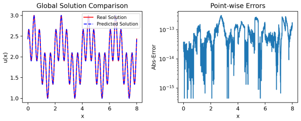
The discovery the paper is trying to establish is that separating basis generation from solution fitting makes high-accuracy neural PDE solving cheap. In each subdomain, a subspace neural network outputs $M$ basis functions and represents the local solution as $\hat u = \sum_{j=1}^M \beta_j \phi_j$; training updates only the network weights, with $\beta$ fixed to 1, and then the assembled least-squares system determines $\beta$ from three sources: interior equation residuals, boundary conditions, and $C^k$ interface conditions between adjacent subdomains. On the reported benchmarks this two-step fit reaches $L^2$ errors of $4.98\times10^{-11}$ (1D Helmholtz), $4.94\times10^{-12}$ (2D Poisson), $2.33\times10^{-11}$ (parabolic), $2.45\times10^{-7}$ (singular-perturbed boundary layer), and $9.49\times10^{-10}$ (nonlinear Helmholtz), with a best 1D Helmholtz error of $9.49\times10^{-13}$ at 16 subdomains, and the Newton version on viscous Burgers reaches $4.19\times10^{-10}$. The paper interprets these numbers as showing that domain decomposition and subspace representation, not network depth or long training, are the decisive accuracy ingredients.
Load-bearing premise
The load-bearing premise is that basis functions trained with $\beta=1$ against the bare PDE residual form a subspace rich enough and stable enough for the later least-squares coefficient solve to deliver the advertised $10^{-10}$ to $10^{-13}$ accuracy; the paper provides no analysis connecting that training objective to the final fit.
Editorial extensions
If this is right
- For a fixed trained basis, changing the source term or boundary data in a linear problem reduces to re-solving the least-squares system for the coefficients, so parametric sweeps avoid retraining the networks.
- Because each subdomain trains independently, the method supports straightforward parallel training, and increasing resolution can be done by adding subdomains rather than deepening the network.
- For nonlinear problems, Picard and Newton iterations act on the small coefficient vector with the basis frozen, so per-iteration cost is governed by the least-squares solve rather than by network backpropagation.
- The experiments show accuracy improving as the number of subdomains increases up to a limit set by the number of collocation points per subdomain, so domain count and subspace dimension are practical accuracy controls.
Reading between the lines
- A likely reading, not stated in the paper, is that most of the accuracy comes from the overdetermined least-squares fit and the interface constraints rather than from the trained hidden layers; the paper's own tables show that zero hidden layers is sometimes the most accurate configuration, which makes a clean testable comparison between trained bases and untrained random-feature bases.
- The $C^k$ interface condition scales with equation order: a fourth-order PDE would require $C^3$ continuity across interfaces, adding derivative rows to the global system and potentially eroding the efficiency advantage reported here.
- The reported errors are all against smooth, manufactured exact solutions; a natural stress test is a nonsmooth or shock-forming solution where a smooth residual-trained basis may require many subdomains or fail to represent the discontinuity.
- The two-stage structure invites an adaptive loop, not present in the paper: after the coefficient solve, measure the residual locally and refine subdomains or enlarge the subspace where the residual is largest.
Editorial analysis
A structured set of objections, weighed in public.
Referee Report
Summary. The manuscript proposes DD-SNN, a domain-decomposition variant of the subspace neural network (SNN) method for linear and nonlinear PDEs. Local SNNs are trained independently on each subdomain by minimizing the PDE residual with the combination coefficients fixed to 1; afterwards, the coefficients are recovered by a least-squares solve of a global system that enforces the PDE, boundary conditions, and C^k interface continuity. Nonlinear problems are handled by Picard and Newton iterations on the coefficients. The paper reports extensive 1D/2D benchmarks (linear and nonlinear Helmholtz, Poisson, parabolic, singular perturbation, viscous Burgers) and claims errors down to 1e-13 with substantially lower training cost than PINNs, DGM, DRM, ELM, and LocELM.
Significance. If the numerical claims hold, the method is a practical contribution: the per-subdomain training is embarrassingly parallel, the coefficient solve is a standard least-squares problem, and the reported errors on smooth manufactured solutions are impressively low. The paper's strengths are the breadth of ablations (subdomain count, subspace dimension, hidden-layer count, sampling method, random seed) and the consistent reporting of errors, epochs, and CPU times. However, the central accuracy claim is supported only by selected benchmark configurations: there is no convergence or conditioning analysis, the interface continuity order used in the experiments is never stated, and the baseline timing comparisons are not controlled. The contribution is promising but needs additional evidence before the headline claims can be accepted.
major comments (4)
- [Section 2 (Eq. (3)) and Section 3 (Eqs. (13)-(15))] The load-bearing path to the advertised accuracy is the two-stage construction: basis functions are trained with beta fixed to 1 and stopping tolerance epsilon=1e-3, and then the global coefficient vector is obtained by the least-squares solve (15). The paper provides no analysis or diagnostic showing that this trained subspace is well conditioned for that solve. In particular, the numerical rank, smallest singular value, or condition number of the matrix A in Eq. (13) is never reported. Without such information, the 1e-11 to 1e-13 errors in Tables 1, 6, 21, and 25 may reflect the chosen collocation grid or initialization rather than a property of the method. Please add a conditioning/rank analysis of A for the reported configurations, or an ablation that varies the fixed beta value during basis training and reports the resulting conditioning and errors.
- [Section 2 (Eq. (5)) and Section 5] The continuity order k_s is a free parameter of the method, but no numerical experiment in Section 5 states which k_s was used. Since the global system (13) is assembled from interface equations of the form (12), the reported accuracy depends directly on this choice, and the omission makes the experiments irreproducible. Please state k_s for each benchmark and justify the choice from the PDE order; the remark following Eq. (5) that a highest derivative k_s requires C^{k_s-1} also needs to be reconciled with the C^k notation used elsewhere.
- [Section 5 (Tables 1, 6, 11, 16, 21, 25)] The comparison baselines do not currently support the claim of 'significantly reducing computational costs.' PINNs, DGM, and DRM are run for a fixed 50,000 epochs without tuning, and CPU times are measured across different implementations (e.g., DEEPXDE for PINNs), so the time comparisons may reflect implementation and hardware rather than algorithmic efficiency. Please provide convergence curves for the baselines, report whether they have plateaued, use equivalent implementations/hardware for all methods, and tune baseline hyperparameters or justify why the chosen settings are representative.
- [Abstract and Section 5] The claim that errors 'reach up to 10^-13' overstates the evidence. The 1e-13 accuracy appears only for selected configurations (e.g., Table 2 with 16 subdomains and Table 8 with zero hidden layers), while the singular-perturbation problem in Table 16 saturates around 1e-7 and the nonlinear examples in Tables 21 and 25 are at roughly 1e-9 to 1e-10. The abstract should report the range of errors across benchmarks or state the conditions under which 1e-13 is achieved, and the conclusion should not imply that all tested problems reach that accuracy.
minor comments (5)
- [Eq. (2a)] The normalization formula appears garbled: the expression '2 bkx−akx · (x − akx) − 1 2 bk t −ak t · (t − ak t ) − 1' is missing parentheses and superscripts, and it is unclear how the temporal coordinate is treated in steady-state problems where no time direction exists.
- [Section 5.1.3 (Table 11)] The text says DD-SNN achieves its result with 'an average of 135 epochs,' while Table 11 reports 98 epochs for the same configuration; please correct the inconsistency.
- [Tables 6 and 9] For the two-dimensional Poisson equation with 16 subdomains and uniform sampling, Table 6 reports an L_infinity error of 6.61e-11 while Table 9 reports 2.02e-10 for what appears to be the same configuration; please verify which value is correct.
- [Section 5.1.3 (Table 11)] The text states that the PINN L2 error is 9.96e-3, but Table 11 reports 2.29e-2 for PINN; please correct the text or the table.
- [References in Section 1] Reference [19] is cited for two different works in the introduction: once for 'compensated deep Ritz methods' and once for 'randomized neural network with Petrov-Galerkin methods'; please renumber the references so each citation points to the intended work.
Circularity Check
No significant circularity: DD-SNN is validated against manufactured exact solutions, and its two-stage residual-minimization/least-squares construction is a standard projection method rather than a self-referential prediction.
full rationale
The derivation chain is self-contained. Basis functions are trained by minimizing the PDE residual with beta=1 (Eq. 3), and the coefficients are then obtained by least-squares enforcement of the same PDE, boundary, and interface equations (Eqs. 13-15). This is a collocation/least-squares projection over the trained subspace; the target solution enters only through the source term f and boundary data g, which are legitimate problem inputs. All headline errors (e.g., 4.98e-11 in Table 1, 1e-13 in Table 2) are measured against exact solutions chosen independently of the algorithm, so the validation is external. The only self-citation is Ref. [8] (Xu and Sheng) for the SNN architecture; the paper restates the propagation equations and does not invoke any uniqueness theorem or prior accuracy claim from [8] as load-bearing. The beta=1 basis-training step and the later least-squares solve are both parts of the algorithm, not a fitted parameter renamed as a prediction. Conditioning or representability concerns about the least-squares matrix A (Eq. 13) would be correctness/robustness questions, not circularity.
Assumptions & free parameters
free parameters (4)
- Subspace dimension M per subdomain =
100, 200, or 300 depending on experiment
- Number of subdomains Nk =
4, 8, 9, 16, 25, or 32 per experiment
- Basis-training stopping tolerance epsilon =
1e-3
- Nonlinear iteration tolerances epsilon_non =
1e-6 for Helmholtz, 1e-12/1e-13 for Burgers
assumptions (4)
- domain assumption Neural networks of the chosen depth and width can approximate the local PDE solution well enough inside each subdomain.
- ad hoc to paper Basis functions trained by minimizing the PDE residual with beta=1 remain good bases for the later coefficient solve.
- domain assumption Imposing C^k continuity on subdomain interfaces is sufficient for a global solution of the PDE.
- domain assumption Picard and Newton iterations on the coefficients converge for the tested nonlinear problems.
Cite this review
Pith. "Pith review of Domain Decomposition Subspace Neural Network Method for Solving Linear and Nonlinear Partial Differential Equations." pith.science (2026). https://pith.science/paper/MSSB3D25
@misc{pith2026250520818,
  author       = {Pith},
  title        = {Pith review of: Domain Decomposition Subspace Neural Network Method for Solving Linear and Nonlinear Partial Differential Equations},
  year         = {2026},
  howpublished = {\url{https://pith.science/paper/MSSB3D25}},
  note         = {Machine review of arXiv:2505.20818}
}
abstract
This paper proposes a domain decomposition subspace neural network method for efficiently solving linear and nonlinear partial differential equations. By combining the principles of domain decomposition and subspace neural networks, the method constructs basis functions using neural networks to approximate PDE solutions. It imposes $C^k$ continuity conditions at the interface of subdomains, ensuring smoothness across the global solution. Nonlinear PDEs are solved using Picard and Newton iterations, analogous to classical methods. Numerical experiments demonstrate that our method achieves exceptionally high accuracy, with errors reaching up to $10^{-13}$, while significantly reducing computational costs compared to existing approaches, including PINNs, DGM, DRM. The results highlight the method's superior accuracy and training efficiency.
Figures


Figures from the paper (10 more)


Reference graph
Works this paper leans on
-
[8]
Z. Xu, Z. Sheng, Subspace method based on neural networks for solving the partial differential equation, arXiv preprint arXiv:2404.08223 (2024)
work page Pith review arXiv 2024
-
[10]
S. Dong, Z. Li, Local extreme learning machines and domain decom- position for solving linear and nonlinear partial differential equations, Computer Methods in Applied Mechanics and Engineering 387 (2021) 114129
2021
-
[1]
L. C. Evans, Partial Differential Equations, American Mathematical So- ciety, 2022
work page 2022
-
[2]
J. H. Ferziger, Computational Methods for Fluid Dynamics, Springer, 2020
work page 2020
-
[3]
R. L. Taylor, O. C. Zienkiewicz, The Finite Element Method, Butterworth-Heinemann, 2013
work page 2013
-
[4]
J. P. Boyd, Chebyshev and Fourier Spectral Methods, Courier Corpo- ration, 2001
work page 2001
- [5]
-
[6]
J. Chen, X. Chi, Z. Yang, Bridging traditional and machine learning- based algorithms for solving PDEs: the random feature method, Journal of Machine Learning 1(3) (2022) 268-298
work page 2022
Show all 27 references
-
[7]
M. Yang, J. T. Foster, Multi-output physics-informed neural networks for forward and inverse PDE problems with uncertainties, Computer Methods in Applied Mechanics and Engineering 402 (2022) 115041, DOI: 10.1016/j.cma.2022.115041. 40
2022
-
[9]
Huang, Q
G. Huang, Q. Zhu, C. Siew, Extreme learning machine: theory and applications, Neurocomputing 70(1-3) (2006) 489-501
2006
-
[11]
Y. Peng, D. Hu, Z.-Q. J. Xu, A non-gradient method for solving ellip- tic partial differential equations with deep neural networks, Journal of Computational Physics 472 (2023) 111690
2023
-
[12]
Basir, I
S. Basir, I. Senocak, Critical investigation of failure modes in physics- informed neural networks, AIAA SCITECH 2022 Forum, 2022
2022
-
[13]
J. Y. Nguwi, G. Penent, N. Privault, A deep branching solver for fully nonlinear partial differential equations, Journal of Computational Physics 499 (2024) 112712
2024
-
[14]
J. Zuo, J. Yang, Approximation properties of residual neural networks for fractional differential equations, Communications in Nonlinear Sci- ence and Numerical Simulation 125 (2023) 107399
2023
-
[15]
Bai, G.-R
J. Bai, G.-R. Liu, A. Gupta, L. Alzubaidi, X.-Q. Feng, Y. Gu, Physics- informed radial basis network (PIRBN): A local approximating neural network for solving nonlinear partial differential equations, Computer Methods in Applied Mechanics and Engineering 415 (2023) 116290, DOI...
2023
-
[16]
Y. Xie, Y. Ma, Y. Wang, Automatic boundary fitting framework of boundary dependent physics-informed neural network solving partial dif- ferential equation with complex boundary conditions, Computer Meth- ods in Applied Mechanics and Engineering 414 (2023) 116139
2023
-
[17]
Dekhovich, M
A. Dekhovich, M. H. F. Sluiter, D. M. J. Tax, M. A. Bessa, iPINNs: Incremental learning for Physics-informed neural networks, Engineering with Computers 41(1) (2025) 389-402, DOI: 10.1007/s00366-024-02010- 1. 41
2025 doi
-
[18]
C. Liu, H. A. Wu, cv-PINN: Efficient learning of variational physics- informed neural network with domain decomposition, Extreme Mechan- ics Letters 63 (2023) 102051
2023
-
[19]
Shang, F
Y. Shang, F. Wang, J. Sun, Randomized neural network with Petrov–Galerkin methods for solving linear and nonlinear partial differ- ential equations, Communications in Nonlinear Science and Numerical Simulation 127 (2023) 107518
2023
-
[20]
H. Cobb, H. Lee, Y. Liu, Solving Maxwell’s Equation in 2D with Neural Networks with Local Converging Inputs, arXiv preprint arXiv:2302.02860 (2023)
2023 arXiv
-
[21]
Z. Lin, Y. Wang, H. Xie, Adaptive Neural Network Subspace Method for Solving Partial Differential Equations with High Accuracy, arXiv preprint arXiv:2412.02586 (2024)
2024 arXiv
-
[22]
Y. Wang, H. Xie, Computing multi-eigenpairs of high-dimensional eigen- value problems using tensor neural networks, Journal of Computational Physics 506 (2024) 112928
2024
-
[23]
H. Li, X. Ye, P. Jiang, G. Qin, T. Wang, Local neural operator for solv- ing transient partial differential equations on varied domains, Computer Methods in Applied Mechanics and Engineering 427 (2024) 117062, DOI: 10.1016/j.cma.2024.117062
2024
-
[24]
Y. Wang, L. Zhong, NAS-PINN: Neural architecture search-guided physics-informed neural network for solving PDEs, Journal of Compu- tational Physics 496 (2024) 112603
2024
-
[25]
J. W. Siegel, Q. Hong, X. Jin, W. Hao, J. Xu, Greedy training algorithms for neural networks and applications to PDEs, Journal of Computational Physics 484 (2023) 112084, DOI: 10.1016/j.jcp.2023.112084
2023
-
[26]
Z. Ye, X. Huang, L. Chen, H. Liu, Z. Wang, B. Dong, Pdeformer: To- wards a foundation model for one-dimensional partial differential equa- tions, arXiv preprint arXiv:2402.12652 (2024)
2024 arXiv
-
[27]
A. D. Jagtap, G. E. Karniadakis, Extended physics-informed neural networks (XPINNs): A generalized space-time domain decomposition based deep learning framework for nonlinear partial differential equa- tions, Communications in Computational Physics 28(5) (2020). 42
2020
Reviewed August 7, 2026 · model on record in the stance chip above.
Discussion (0). Continue with ORCID to comment.