Ion firehose and ion cyclotron instability with subtracted-Kappa distributions
Pith reviewed 2026-06-26 02:01 UTC · model grok-4.3
The pith
Enhancing the loss-cone feature in subtracted-Kappa ion distributions decreases growth rates of the ion firehose instability while increasing those of the ion cyclotron instability.
A machine-rendered reading of the paper's core claim, the machinery that carries it, and where it could break.
Core claim
Numerical solutions of the dispersion relation demonstrate that, for ions described by subtracted-Kappa distributions, increasing the loss-cone feature leads to a decrease in the growth rates of the firehose instability when T_i⊥ < T_i∥ and to an increase in the growth rates of the ion-cyclotron instability when T_i⊥ > T_i∥. The solutions further indicate that electron thermal anisotropy and the presence of electron drift velocity influence the growth rates in both cases.
What carries the argument
The subtracted-Kappa distribution for ions, which incorporates a tunable loss-cone feature into a bi-Kappa form and is used to close the dispersion relation for parallel electromagnetic waves.
If this is right
- Increasing the loss-cone parameter stabilizes the plasma against firehose growth when parallel ion temperature is higher.
- Increasing the loss-cone parameter destabilizes the plasma through higher ion-cyclotron growth when perpendicular ion temperature is higher.
- Electron temperature anisotropy alters the growth rates of both instabilities.
- Electron drift velocity shifts the thresholds and growth rates for both instabilities.
Where Pith is reading between the lines
- The opposite response of the two instabilities to the same distribution feature may require separate stability criteria when modeling wave activity in regions with varying ion anisotropies.
- Predictions of wave spectra in magnetized plasmas could change if loss-cone parameters are adjusted to match observed distributions rather than assumed forms.
- The results suggest that loss-cone strength might serve as a control parameter when testing how different ion distributions affect overall plasma stability.
Load-bearing premise
The subtracted-Kappa distributions with the chosen parameters accurately represent the ion velocity distributions in the space plasma environments under study.
What would settle it
Spacecraft measurements of ion velocity distributions that lack the modeled loss-cone feature or exhibit growth rates for firehose and cyclotron waves whose dependence on the loss-cone parameter contradicts the numerical solutions.
Figures
read the original abstract
In the present paper we discuss numerical solutions of the dispersion relation for electromagnetic waves propagating along the lines of an ambient magnetic field, considering parameters representative of space plasma environments, and considering the ion population described by a subtracted-Kappa distribution. We consider situations in which the ion thermal anisotropy is such that $T_{i\perp}<T_{i\parallel}$, and investigate the effect of some parameters associated to the subtracted-Kappa distribution on the ion firehose instability. We also consider situations in which $T_{i\perp}>T_{i\parallel}$, and investigate the effects of the same parameters on the ion-cyclotron instability. For both forms of instability, we also investigate the effect of the thermal anisotropy of the electron distribution, and the effect of the occurrence of a drift velocity in the electron distribution function. Among the results obtained, we show that the increase of the loss-cone feature in a bi-kappa distribution leads to a decrease of the growth rates of the firehose instability, and to an increase of the growth rates of the ion-cyclotron instability.
Editorial analysis
A structured set of objections, weighed in public.
Referee Report
Summary. The manuscript reports numerical solutions of the parallel electromagnetic dispersion relation for ions modeled by subtracted-Kappa distributions with parameters representative of space plasmas. For T_i⊥ < T_i∥ it examines the ion firehose instability and for T_i⊥ > T_i∥ the ion-cyclotron instability, finding that an increase in the loss-cone feature decreases firehose growth rates while increasing ion-cyclotron growth rates; effects of electron anisotropy and electron drift are also considered.
Significance. If the numerical results are robust, the directional dependence of the two instabilities on the loss-cone parameter within the subtracted-Kappa model would provide a concrete, testable prediction for how non-thermal features modulate wave growth in space plasmas. The work performs the exact calculation needed to establish that dependence for the chosen functional form.
major comments (1)
- [Abstract] Abstract (and any Numerical Methods section): the manuscript states that numerical solutions of the dispersion relation were obtained but supplies no information on the integration method, discretization, convergence tests, error estimates, or comparison against known analytic limits (e.g., Maxwellian or bi-Maxwellian cases). Because the central claims rest entirely on the reported growth-rate trends, this omission is load-bearing.
minor comments (1)
- [Abstract] Abstract: the phrases 'subtracted-Kappa distribution' and 'bi-kappa distribution' appear; a brief clarification of their precise relationship (or a reference to the defining equation) would aid readability.
Simulated Author's Rebuttal
We thank the referee for their detailed review and constructive suggestion. The single major comment identifies a genuine omission in the presentation of our numerical results. We address it directly below and will revise the manuscript accordingly.
read point-by-point responses
-
Referee: [Abstract] Abstract (and any Numerical Methods section): the manuscript states that numerical solutions of the dispersion relation were obtained but supplies no information on the integration method, discretization, convergence tests, error estimates, or comparison against known analytic limits (e.g., Maxwellian or bi-Maxwellian cases). Because the central claims rest entirely on the reported growth-rate trends, this omission is load-bearing.
Authors: We agree that the absence of numerical-method details weakens the manuscript. In the revised version we will insert a dedicated Numerical Methods subsection (or appendix) that specifies: (i) the quadrature/integration scheme employed to evaluate the velocity-space integrals in the dispersion relation, (ii) the discretization parameters (grid resolution, cutoff velocities, number of points), (iii) convergence tests performed by varying those parameters, (iv) error estimates or tolerance criteria used to accept a root, and (v) benchmark comparisons against the known analytic limits for Maxwellian and bi-Maxwellian distributions. These additions will be referenced from the abstract and from the results sections. revision: yes
Circularity Check
No significant circularity detected
full rationale
The paper computes numerical solutions of the parallel electromagnetic dispersion relation for a subtracted-Kappa ion distribution (with parameters stated as representative of space plasmas). The central claims concern directional trends in growth rates as functions of loss-cone feature, anisotropy, and electron parameters. These are direct numerical outputs of the dispersion integral for the chosen functional form; no parameter is fitted to a subset of results and then re-predicted, no self-citation supplies a uniqueness theorem or ansatz that forces the outcome, and no renaming of known results occurs. The derivation chain is self-contained against external benchmarks and does not reduce to its inputs by construction.
Axiom & Free-Parameter Ledger
Reference graph
Works this paper leans on
-
[1]
These values can be considered as representative of space plasma environments [31]
0 × 10− 4, with vi∥ being the ion parallel thermal veloc- ity, and vA = B0/ √ 4πn i0mi being the Alfv´ en velocity. These values can be considered as representative of space plasma environments [31]. We also consider for all cases Te∥ = Ti∥. Moreover, we assume v∗ = vA and Ω ∗ = Ω i, so that z = ω/ Ω i, and q∥ = k∥vA/ Ω i. We then solve the dispersion rel...
-
[2]
15 0 0 . 2 0 . 4 0 . 6 0 . 8 1 1 . 2 1 . 4 1 . 6 1 . 8 ∆ i = 0. 0 ω i/ Ω i k∥vA/ Ω i βi = 0. 0βi = 0. 2βi = 0. 4βi = 0. 6βi = 0. 8 0
-
[3]
5 0 0 . 2 0 . 4 0 . 6 0 . 8 1 1 . 2 1 . 4 1 . 6 1 . 8 ∆ i = 0. 0 ω r/ Ω i k∥vA/ Ω i βi = 0. 0βi = 0. 2βi = 0. 4βi = 0. 6βi = 0. 8 − 0. 1 − 0. 05 0
-
[4]
15 0 0 . 2 0 . 4 0 . 6 0 . 8 1 1 . 2 1 . 4 1 . 6 1 . 8 ∆ i = 0. 5 ω i/ Ω i k∥vA/ Ω i βi = 0. 0βi = 0. 2βi = 0. 4βi = 0. 6βi = 0. 8 0
-
[5]
8 2 0 0 . 2 0 . 4 0 . 6 0 . 8 1 1 . 2 1 . 4 1 . 6 1 . 8 ∆ i = 0. 5 ω r/ Ω i k∥vA/ Ω i βi = 0. 0βi = 0. 2βi = 0. 4βi = 0. 6βi = 0. 8 − 0. 1 − 0. 05 0
-
[6]
15 0 0 . 2 0 . 4 0 . 6 0 . 8 1 1 . 2 1 . 4 1 . 6 1 . 8 ∆ i = 0. 9 ω i/ Ω i k∥vA/ Ω i βi = 0. 0βi = 0. 2βi = 0. 4βi = 0. 6βi = 0. 8 0
-
[7]
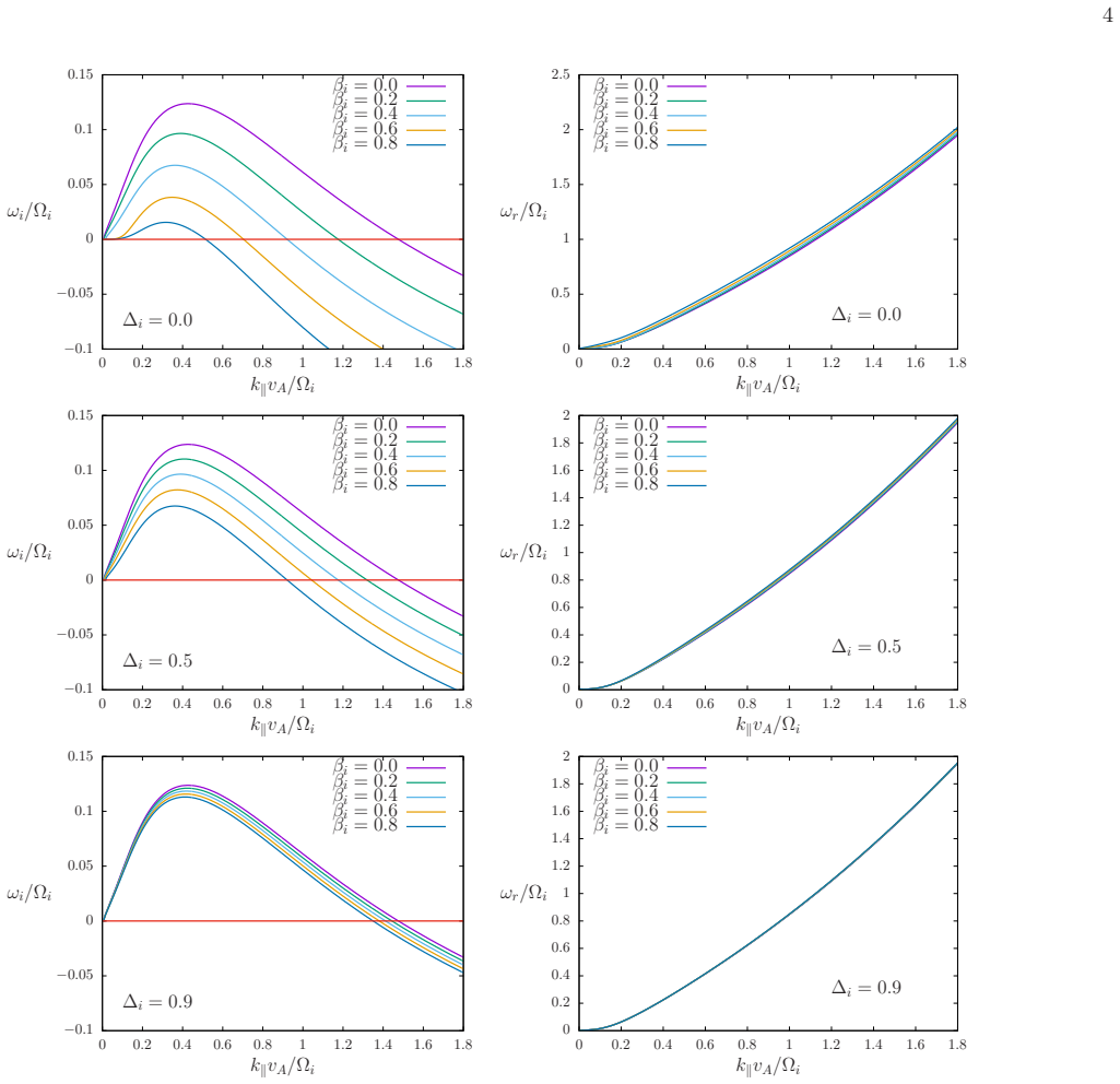
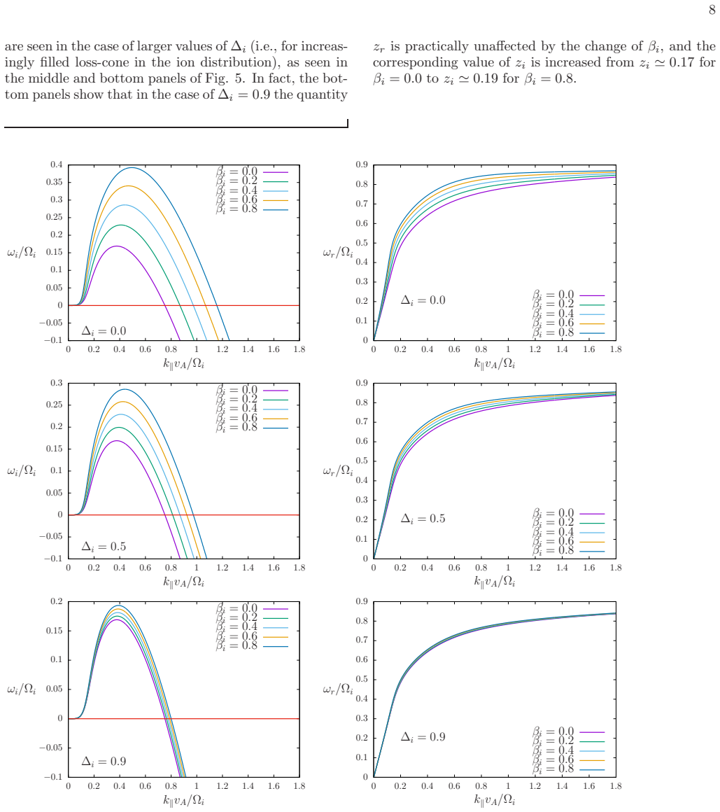
8 2 0 0 . 2 0 . 4 0 . 6 0 . 8 1 1 . 2 1 . 4 1 . 6 1 . 8 ∆ i = 0. 9 ω r/ Ω i k∥vA/ Ω i βi = 0. 0βi = 0. 2βi = 0. 4βi = 0. 6βi = 0. 8 Figure 1: The left panels show the imaginary part of the norma lized frequency of unstable parallel propagating electrom agnetic waves, zi, vs. normalized wave number q∥. The panels to the right show the corresponding real pa...
-
[8]
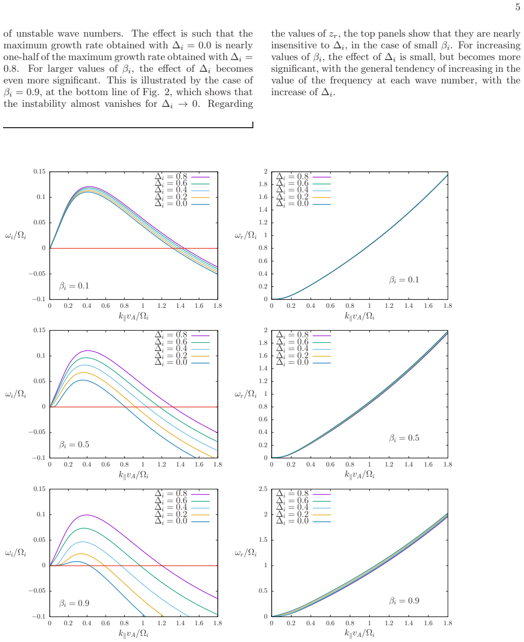
For larger values of βi, the effect of ∆ i becomes even more significant
8. For larger values of βi, the effect of ∆ i becomes even more significant. This is illustrated by the case of βi = 0 . 9, at the bottom line of Fig. 2, which shows that the instability almost vanishes for ∆ i → 0. Regarding the values of zr, the top panels show that they are nearly insensitive to ∆ i, in the case of small βi. For increasing values of βi, ...
-
[9]
15 0 0 . 2 0 . 4 0 . 6 0 . 8 1 1 . 2 1 . 4 1 . 6 1 . 8 βi = 0. 1 ω i/ Ω i k∥vA/ Ω i ∆ i = 0. 8∆ i = 0. 6∆ i = 0. 4∆ i = 0. 2∆ i = 0. 0 0
-
[10]
8 2 0 0 . 2 0 . 4 0 . 6 0 . 8 1 1 . 2 1 . 4 1 . 6 1 . 8 βi = 0. 1 ω r/ Ω i k∥vA/ Ω i ∆ i = 0. 8∆ i = 0. 6∆ i = 0. 4∆ i = 0. 2∆ i = 0. 0 − 0. 1 − 0. 05 0
-
[11]
15 0 0 . 2 0 . 4 0 . 6 0 . 8 1 1 . 2 1 . 4 1 . 6 1 . 8 βi = 0. 5 ω i/ Ω i k∥vA/ Ω i ∆ i = 0. 8∆ i = 0. 6∆ i = 0. 4∆ i = 0. 2∆ i = 0. 0 0
-
[12]
8 2 0 0 . 2 0 . 4 0 . 6 0 . 8 1 1 . 2 1 . 4 1 . 6 1 . 8 βi = 0. 5 ω r/ Ω i k∥vA/ Ω i ∆ i = 0. 8∆ i = 0. 6∆ i = 0. 4∆ i = 0. 2∆ i = 0. 0 − 0. 1 − 0. 05 0
-
[13]
15 0 0 . 2 0 . 4 0 . 6 0 . 8 1 1 . 2 1 . 4 1 . 6 1 . 8 βi = 0. 9 ω i/ Ω i k∥vA/ Ω i ∆ i = 0. 8∆ i = 0. 6∆ i = 0. 4∆ i = 0. 2∆ i = 0. 0 0
-
[14]
5 0 0 . 2 0 . 4 0 . 6 0 . 8 1 1 . 2 1 . 4 1 . 6 1 . 8 βi = 0. 9 ω r/ Ω i k∥vA/ Ω i ∆ i = 0. 8∆ i = 0. 6∆ i = 0. 4∆ i = 0. 2∆ i = 0. 0 Figure 2: The left panels show the imaginary part of the norma lized frequency of unstable parallel propagating electrom agnetic waves, zi, vs. normalized wave number q∥. The panels to the right show the corresponding real ...
-
[15]
12 0 0 . 2 0 . 4 0 . 6 0 . 8 1 1 . 2 1 . 4 1 . 6 1 . 8 βi = 0. 5, ∆ i = 0. 5 ω i/ Ω i k∥vA/ Ω i κi = 2. 5κi = 3. 0κi = 5. 0κi = 10. 0κi = 30. 0 0
-
[16]
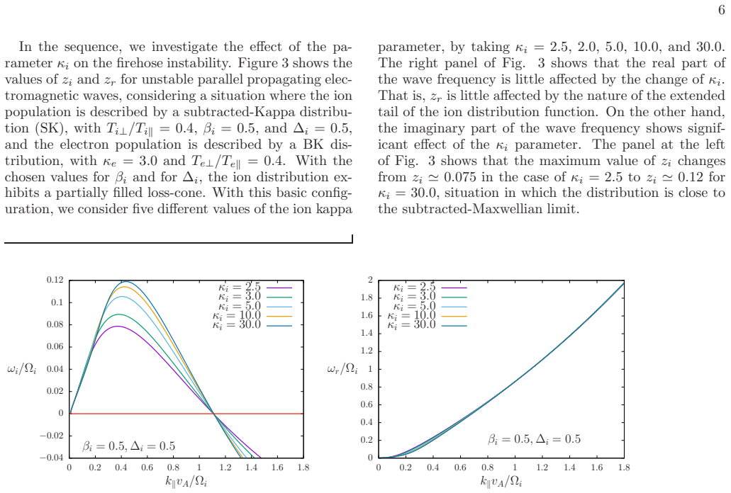
8 2 0 0 . 2 0 . 4 0 . 6 0 . 8 1 1 . 2 1 . 4 1 . 6 1 . 8 βi = 0. 5, ∆ i = 0. 5 ω r/ Ω i k∥vA/ Ω i κi = 2. 5κi = 3. 0κi = 5. 0κi = 10. 0κi = 30. 0 Figure 3: The left panel shows the imaginary part of the norma lized frequency of unstable parallel propagating electrom agnetic waves, zi, vs. normalized wave number q∥. The panels to the right show the correspo...
-
[17]
1 0 0 . 2 0 . 4 0 . 6 0 . 8 1 1 . 2 1 . 4 1 . 6 1 . 8 ∆ i = 0. 5, β i = 0. 5 ω i/ Ω i k∥vA/ Ω i Ued = 0. 0Ued = 0. 1Ued = 0. 2Ued = 0. 3Ued = 0. 4 0
-
[18]
5 3 0 0 . 2 0 . 4 0 . 6 0 . 8 1 1 . 2 1 . 4 1 . 6 1 . 8 ∆ i = 0. 5, β i = 0. 5 ω r/ Ω i k∥vA/ Ω i Ued = 0. 0Ued = 0. 1Ued = 0. 2Ued = 0. 3Ued = 0. 4 − 0. 04 − 0. 02 0
-
[19]
16 0 0 . 2 0 . 4 0 . 6 0 . 8 1 1 . 2 1 . 4 1 . 6 1 . 8 βi = 0. 5, ∆ i = 0. 5 ω i/ Ω i k∥vA/ Ω i Te⊥ /T e∥ = 0. 2Te⊥ /T e∥ = 0. 4Te⊥ /T e∥ = 0. 6Te⊥ /T e∥ = 0. 8Te⊥ /T e∥ = 1. 0 0
-
[20]
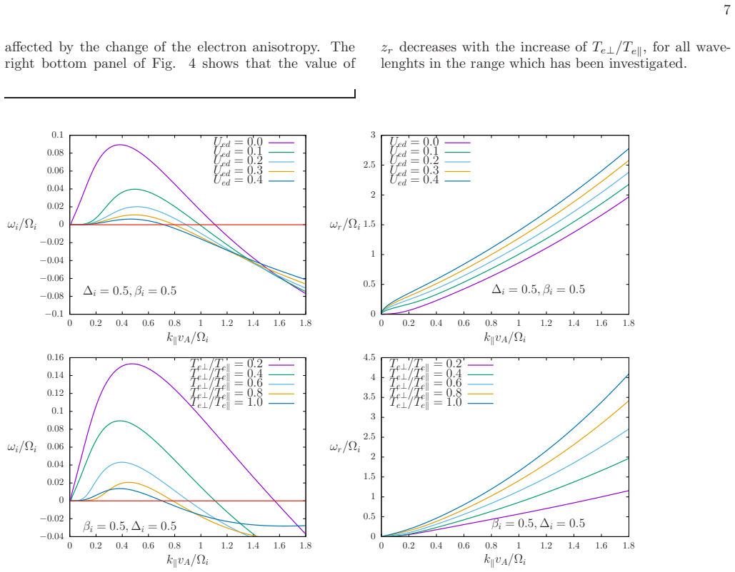
5 0 0 . 2 0 . 4 0 . 6 0 . 8 1 1 . 2 1 . 4 1 . 6 1 . 8 βi = 0. 5, ∆ i = 0. 5 ω r/ Ω i k∥vA/ Ω i Te⊥ /T e∥ = 0. 2Te⊥ /T e∥ = 0. 4Te⊥ /T e∥ = 0. 6Te⊥ /T e∥ = 0. 8Te⊥ /T e∥ = 1. 0 Figure 4: The left panels show the imaginary part of the norma lized frequency of unstable parallel propagating electrom agnetic waves, zi, vs. normalized wave number q∥. The panels...
-
[21]
4 0 0 . 2 0 . 4 0 . 6 0 . 8 1 1 . 2 1 . 4 1 . 6 1 . 8 ∆ i = 0. 0 ω i/ Ω i k∥vA/ Ω i βi = 0. 0βi = 0. 2βi = 0. 4βi = 0. 6βi = 0. 8 0
-
[22]
9 0 0 . 2 0 . 4 0 . 6 0 . 8 1 1 . 2 1 . 4 1 . 6 1 . 8 ∆ i = 0. 0 ω r/ Ω i k∥vA/ Ω i βi = 0. 0βi = 0. 2βi = 0. 4βi = 0. 6βi = 0. 8 − 0. 1 − 0. 05 0
-
[23]
3 0 0 . 2 0 . 4 0 . 6 0 . 8 1 1 . 2 1 . 4 1 . 6 1 . 8 ∆ i = 0. 5 ω i/ Ω i k∥vA/ Ω i βi = 0. 0βi = 0. 2βi = 0. 4βi = 0. 6βi = 0. 8 0
-
[24]
9 0 0 . 2 0 . 4 0 . 6 0 . 8 1 1 . 2 1 . 4 1 . 6 1 . 8 ∆ i = 0. 5 ω r/ Ω i k∥vA/ Ω i βi = 0. 0βi = 0. 2βi = 0. 4βi = 0. 6βi = 0. 8 − 0. 1 − 0. 05 0
-
[25]
2 0 0 . 2 0 . 4 0 . 6 0 . 8 1 1 . 2 1 . 4 1 . 6 1 . 8 ∆ i = 0. 9 ω i/ Ω i k∥vA/ Ω i βi = 0. 0βi = 0. 2βi = 0. 4βi = 0. 6βi = 0. 8 0
-
[26]
9 0 0 . 2 0 . 4 0 . 6 0 . 8 1 1 . 2 1 . 4 1 . 6 1 . 8 ∆ i = 0. 9 ω r/ Ω i k∥vA/ Ω i βi = 0. 0βi = 0. 2βi = 0. 4βi = 0. 6βi = 0. 8 Figure 5: The left panels show the imaginary part of the norma lized frequency of unstable parallel propagating electrom agnetic waves, zi, vs. normalized wave number q∥. The panels to the right show the corresponding real part...
-
[27]
25 0 0 . 2 0 . 4 0 . 6 0 . 8 1 1 . 2 1 . 4 1 . 6 1 . 8 βi = 0. 1 ω i/ Ω i k∥vA/ Ω i ∆ i = 0. 8∆ i = 0. 6∆ i = 0. 4∆ i = 0. 2∆ i = 0. 0 0
-
[28]
9 0 0 . 2 0 . 4 0 . 6 0 . 8 1 1 . 2 1 . 4 1 . 6 1 . 8 βi = 0. 1 ω r/ Ω i k∥vA/ Ω i ∆ i = 0. 8∆ i = 0. 6∆ i = 0. 4∆ i = 0. 2∆ i = 0. 0 − 0. 1 − 0. 05 0
-
[29]
35 0 0 . 2 0 . 4 0 . 6 0 . 8 1 1 . 2 1 . 4 1 . 6 1 . 8 βi = 0. 5 ω i/ Ω i k∥vA/ Ω i ∆ i = 0. 8∆ i = 0. 6∆ i = 0. 4∆ i = 0. 2∆ i = 0. 0 0
-
[30]
9 0 0 . 2 0 . 4 0 . 6 0 . 8 1 1 . 2 1 . 4 1 . 6 1 . 8 βi = 0. 5 ω r/ Ω i k∥vA/ Ω i ∆ i = 0. 8∆ i = 0. 6∆ i = 0. 4∆ i = 0. 2∆ i = 0. 0 − 0. 1 0
-
[31]
4 0 0 . 2 0 . 4 0 . 6 0 . 8 1 1 . 2 1 . 4 1 . 6 1 . 8 βi = 0. 9 ω i/ Ω i k∥vA/ Ω i ∆ i = 0. 8∆ i = 0. 6∆ i = 0. 4∆ i = 0. 2∆ i = 0. 0 0
-
[32]
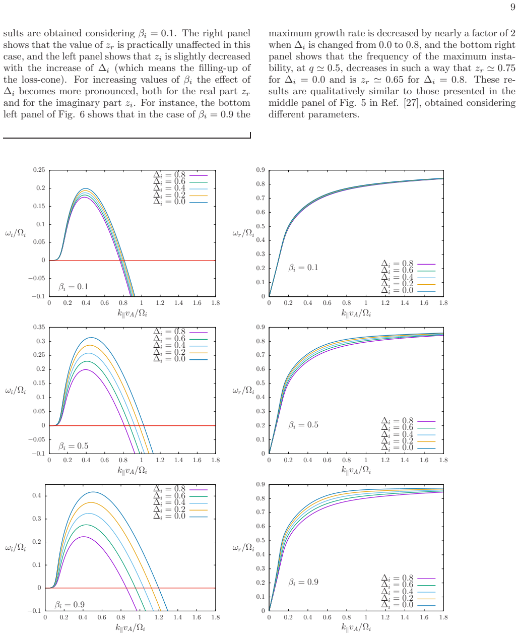
9 0 0 . 2 0 . 4 0 . 6 0 . 8 1 1 . 2 1 . 4 1 . 6 1 . 8 βi = 0. 9 ω r/ Ω i k∥vA/ Ω i ∆ i = 0. 8∆ i = 0. 6∆ i = 0. 4∆ i = 0. 2∆ i = 0. 0 Figure 6: The left panels show the imaginary part of the norma lized frequency of unstable parallel propagating electrom agnetic waves, zi, vs. normalized wave number q∥. The panels to the right show the corresponding real ...
-
[33]
3 0 0 . 2 0 . 4 0 . 6 0 . 8 1 1 . 2 1 . 4 1 . 6 1 . 8 βi = 0. 5, ∆ i = 0. 5 ω i/ Ω i k∥vA/ Ω i κi = 2. 5κi = 3. 0κi = 5. 0κi = 10. 0κi = 30. 0 0
-
[34]
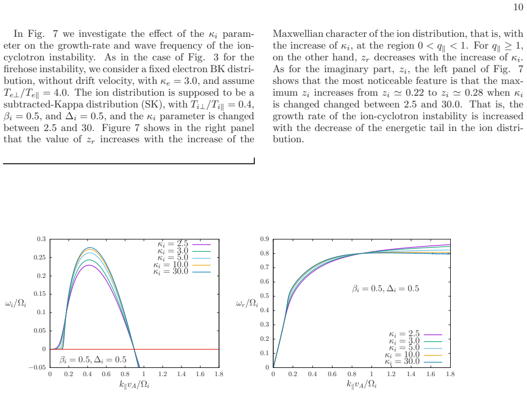
9 0 0 . 2 0 . 4 0 . 6 0 . 8 1 1 . 2 1 . 4 1 . 6 1 . 8 βi = 0. 5, ∆ i = 0. 5 ω r/ Ω i k∥vA/ Ω i κi = 2. 5κi = 3. 0κi = 5. 0κi = 10. 0κi = 30. 0 Figure 7: The left panel shows the imaginary part of the norma lized frequency of unstable parallel propagating electrom agnetic waves, zi, vs. normalized wave number q∥. The panels to the right show the correspond...
-
[35]
25 0 0 . 2 0 . 4 0 . 6 0 . 8 1 1 . 2 1 . 4 1 . 6 1 . 8 ∆ i = 0. 5, β i = 0. 5 ω i/ Ω i k∥vA/ Ω i Ued = 0. 0Ued = 0. 1Ued = 0. 2Ued = 0. 3Ued = 0. 4 0
-
[36]
9 0 0 . 2 0 . 4 0 . 6 0 . 8 1 1 . 2 1 . 4 1 . 6 1 . 8 ∆ i = 0. 5, β i = 0. 5 ω r/ Ω i k∥vA/ Ω i Ued = 0. 0Ued = 0. 1Ued = 0. 2Ued = 0. 3Ued = 0. 4 − 0. 1 0
-
[37]
5 0 0 . 2 0 . 4 0 . 6 0 . 8 1 1 . 2 1 . 4 1 . 6 1 . 8 βi = 0. 5, ∆ i = 0. 5 ω i/ Ω i k∥vA/ Ω i Te⊥ /T e∥ = 5. 0Te⊥ /T e∥ = 4. 0Te⊥ /T e∥ = 3. 0Te⊥ /T e∥ = 2. 0Te⊥ /T e∥ = 1. 0 0
-
[38]
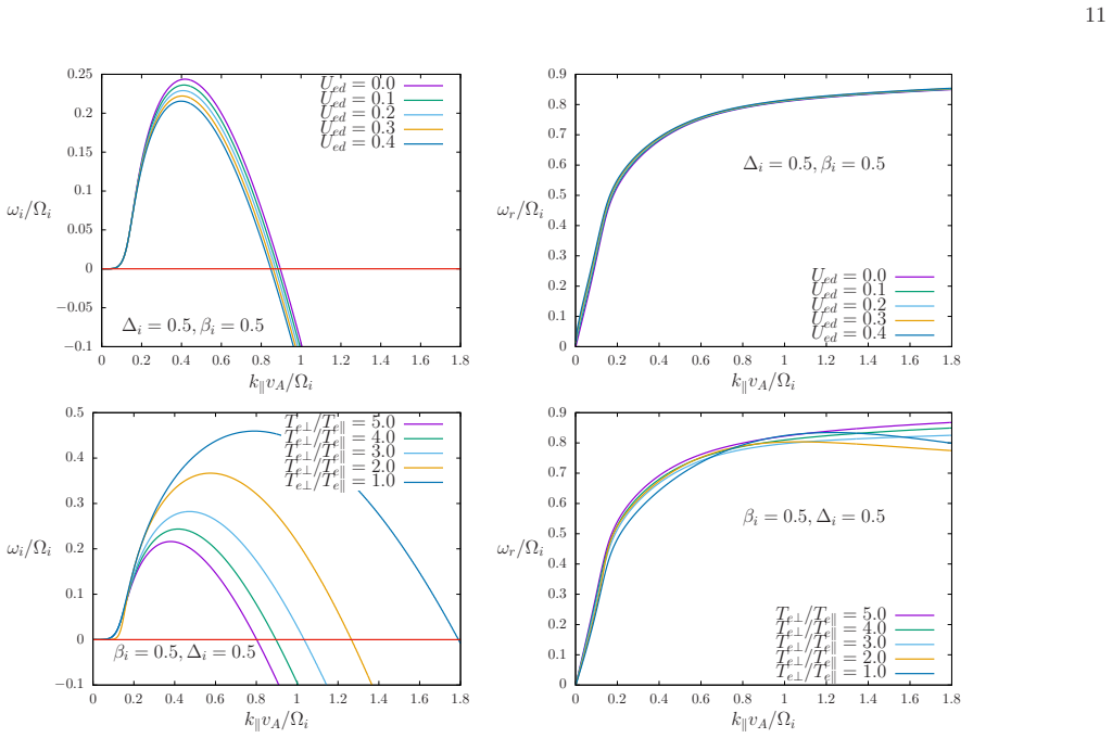
9 0 0 . 2 0 . 4 0 . 6 0 . 8 1 1 . 2 1 . 4 1 . 6 1 . 8 βi = 0. 5, ∆ i = 0. 5 ω r/ Ω i k∥vA/ Ω i Te⊥ /T e∥ = 5. 0Te⊥ /T e∥ = 4. 0Te⊥ /T e∥ = 3. 0Te⊥ /T e∥ = 2. 0Te⊥ /T e∥ = 1. 0 Figure 8: The left panels show the imaginary part of the norma lized frequency of unstable parallel propagating electrom agnetic waves, zi, vs. normalized wave number q∥. The panels...
-
[39]
1, with the upper range of the unstable region changing from q ≃ 0
01 to zi ≃ 0. 1, with the upper range of the unstable region changing from q ≃ 0. 4 to q ≃ 1. 2. When investigating the effect of the parameter κ i, con- trolling the occurrence of an extended power-law tail in the ion distribution, we have seen that the increase of κ i leads to increase in the maximum growth rate of the FH instability, while maintaining t...
2016
-
[40]
W. Pilipp, H. Miggenrieder, M. Montgomery, K.- H. M¨ uhlh¨ auser, H. Rosenbauer, and R. Schwenn, J. Geophys. Res. 92, 1075 (1987), doi: 10.1029/JA092iA02p01075
-
[41]
W. Pilipp, H. Miggenrieder, M. Montgomery, K.- H. M¨ uhlh¨ auser, H. Rosenbauer, and R. Schwenn, J. Geophys. Res. 92, 1093 (1987), doi: 10.1029/JA092iA02p01093
-
[42]
E. Marsch, X.-Z. Ao, and C.-Y. Tu, J. Geophys. Res. 109, A04102, 8p. (2004), doi: 10.1029/2003JA010330
-
[43]
E. Marsch, Living Rev. Solar Phys. 3, 1 (2006), cited 19 Sep. 2006, http://www.livingreviews.org/lrsp-2006-1 , doi: 10.12942/lrsp-2006-1
-
[44]
L. Matteini, S. Landi, P. Hellinger, F. Pantellini, M. Maksimovic, M. Velli, B. E. Goldstein, and E. Marsch, Geophys. Res. Lett. 34, L20105 (2007), doi: 10.1029/2007GL030920
-
[45]
Maksimovic, V
M. Maksimovic, V. Pierrard, and J. F. Lemaire, Astron. Astrophys. 324, 725 (1997)
1997
-
[46]
M. Maksimovic, I. Zouganelis, J.-Y. Chaufray, K. Is- sautier, E. E. Scime, J. E. Littleton, E. Marsch, D. J. McComas, C. Salem, R. P. Lin, and H. El- liot, J. Geophys. Res. 110, A09104, 9p. (2005), doi: 10.1029/2005JA011119
-
[47]
Pierrard, M
V. Pierrard, M. Maksimovic, and J. Lemaire, J. Geophys. Res. 104, 17021 (1999)
1999
-
[48]
V. Pierrard, M. Maksimovic, and J. Lemaire, Astrophys. Space Sci. 277, 195 (2001), doi: 10.1023/A:1012218600882
-
[49]
V. Pierrard and M. Lazar, Solar Phys. 267, 153 (2010), doi: 10.1007/s11207-010-9640-2
-
[50]
S. Stverak, M. Maksimovic, P. M. Travnicek, E. Marsch, A. N. Fazakerley, and E. E. Scime, J. Geophys. Res. 114, A05104, 15p. (2009), doi: 10.1029/2008JA013883
-
[51]
V. M. Vasyliunas, J. Geophys. Res. 73, 2839 (1968), doi: 10.1029/JA073i009p02839
-
[52]
M. P. Leubner, Phys. Plasmas 11, 1308 (2004), doi: 10.1063/1.1667501
-
[53]
D. Summers and R. M. Thorne, Phys. Fluids B 3, 1835 (1991), doi: 10.1063/1.859653
-
[54]
R. L. Mace and M. A. Hellberg, Phys. Plasmas 2, 2098 (1995), doi: 10.1063/1.871296
-
[55]
M. P. Leubner, Astrophys. Space Sci. 282, 573 (2002), doi: 10.1023/A:1020990413487
-
[56]
M. P. Leubner, Astrophys. J. 604, 469 (2004), doi: 10.1086/381867
-
[57]
Z. Ali and M. Sarfraz, Phys. Plasmas 28, 092901 (2021), doi: 10.1063/5.0054768
-
[58]
S. M. Shaaban, M. Lazar, R. F. Wimmer-Schweingruber, and H. Fichtner, Astrophys. J. 918, 37 (2021), doi: 10.3847/1538-4357/ac0f01
-
[59]
A. Micera, E. Boella, A. N. Zhukov, S. M. Shaaban, R. A. Lopez, M. Lazar, and G. Lapenta, Astrophys. J. 893, 130 (2020), doi: 10.3847/1538-4357/ab7faa
-
[60]
Livadiotis, Kappa Distributions: Theory and Applica- tions in Plasmas , Elsevier, Amsterdam, 2017
G. Livadiotis, Kappa Distributions: Theory and Applica- tions in Plasmas , Elsevier, Amsterdam, 2017
2017
-
[61]
Lazar and H
M. Lazar and H. Fichtner, editors, Kappa Distributions: From Observational Evidences via Controversial Predic- tions to a Consistent Theory of Nonequilibrium Plasmas , volume 464 of Astrophysics and Space Science Library , Springer, Cham, 2021
2021
-
[62]
M. Lazar and S. Poedts, Astron. Astrophys. 494, 311 (2009), doi: 10.1051/0004-6361:200811109
-
[63]
2015 Multi- mode quasi-periodic pulsations in a solar flare.Astron
M. Lazar, S. Poedts, and R. Schlickeiser, Astron. Astrophys. 534, A116 (2011), doi: 10.1051/0004- 6361/201116982
-
[64]
M. Lazar, R. Schlickeiser, and S. Poedts, Phys. Plasmas 17, 062112, 5p. (2010), doi: 10.1063/1.3446827
-
[65]
M. S. dos Santos, L. F. Ziebell, and R. Gaelzer, Phys. Plasmas 21, 112102 (2014), doi: 10.1063/1.4900766. 15
-
[66]
D. Summers and S. Stone, Phys. Plasmas 32, 012112 (2025), doi: 10.1063/5.0239741
-
[67]
L. F. Ziebell, R. S. Schneider, M. C. de Juli, and R. Gaelzer, Braz. J. Phys. 38, 297 (2008), doi: 10.1590/S0103-97332008000300002
-
[68]
L. F. Ziebell and R. Gaelzer, Phys. Plasmas 24, 102108 (2017), doi: 10.1063/1.5002136
-
[69]
M. Lazar, H. Fichtner, and P. H. Yoon, Astron. Astro- phys. 589 (2016), doi: 10.1051/0004-6361/201527593
-
[70]
S. P. Gary, Theory of space plasma microinstabilities , Cambridge Atmospheric and Space Science Series, Cam- bridge, New York, 2005
2005
-
[71]
L. F. Ziebell and R. Gaelzer, Braz. J. Phys. 49, 526 (2019), doi: 10.1007/s13538-019-00666-5
discussion (0)
Sign in with ORCID, Apple, or X to comment. Anyone can read and Pith papers without signing in.