REVIEW 2 major objections 6 minor 3 cited by
General superconvergence for kernel-based approximation
T0 review · 2 major / 6 minor · reviewed 2026-08-15 · deepseek-v4-flash
Pith's one-line read Kernel interpolation's superconvergence is governed by adjoint-operator ranges, yielding rates anywhere between the classical and doubled extremes.
desk verdict Solid generalization of superconvergence theory with a clean operator-adjoint framework, but a genuine smoothness-threshold error in the periodic experiment and a missing factor 2 keep it from being fully clean. read the letter →
The pith
A machine-rendered reading of the paper's core claim, the machinery that carries it, and where it could break.
The reading
What carries the argument
The load-bearing object is the adjoint-range condition $v\in A^*(V')$ together with the real $K$-functional of interpolation theory. The proof of Theorem 6 uses the identity $\|v-Pv\|_H=\sup_{\|f\|_H\le1}|\langle v,f-Pf\rangle_H|$, valid for orthogonal projections, and the duality $\langle A^*g,f\rangle_H=g(Af)$; this hands the $\varepsilon$ from the $A$-error to the $H$-error. Corollary 10 then applies the $K$-functional $K(t,v)=\inf_{v_0\in A^*(V')}(\|v-v_0\|_H+t\|v_0\|_{A^*(V')})$ to extract the fractional rate $\varepsilon^\theta$, without any extra structure. In the kernel case, $A$ is the embedding $H(\Omega)\hookrightarrow L_2(\Omega)$, $A^*$ is the Mercer integral operator $T$, and the interpolation spaces are the power spaces $H^{1+\theta}(\Omega)$; for Sobolev kernels these are norm-equivalent to Sobolev spaces of fractional smoothness $(1+\theta)\tau$.
What would settle it
Take a kernel whose Green-function/PDE form is known exactly, such as the reproducing kernel of $W^1_2(0,1)$ with the standard inner product, for which $T(L_2)$ consists of functions $u\in W^2_2(0,1)$ with $u'(0)=u'(1)=0$. Construct $v=Tf$ for a known $f\in L_2(0,1)$, interpolate $v$ at equally spaced interior points, and measure the $L_2$ and $W^1_2$ errors as the fill distance tends to zero. If the rate fails to improve from $h^{\tau}$ to $h^{2\tau}$ (or, for an intermediate member of the interpolation scale, fails to match $\varepsilon^\theta$), the central bound is false; conversely, if a function of the same Sobolev smoothness that violates the boundary conditions achieves the doubled rate, the boundary-condition characterization is incomplete.
Extended reading notes
Core claim
The central discovery is Theorem 6: for any Hilbert space $H$, Banach space $V$, bounded linear operator $A:H\to V$ with adjoint $A^*:V'\to H$, and orthogonal projection $P$, the error bound $\|A(f-Pf)\|_V\le\varepsilon\|f\|_H$ for all $f\in H$ implies $\|v-Pv\|_H\le\|g\|_{V'}\,\varepsilon$ for every $v=A^*g$. Corollary 10 extends this to $v$ in the real interpolation space $(H,A^*(V'))_{\theta,\infty}$, with the rate $\varepsilon^\theta$. In the Mercer setting the interpolation spaces coincide with the power spaces $H^{1+\theta}(\Omega)$, and for Sobolev kernels this yields the Sobolev-norm bound of Corollary 16, interpolating between the standard rate and the doubled rate. The paper also shows that the adjoint of a general operator into $L_p$ is a kernel integral operator, connects the images of such adjoints to Mercer power spaces (Theorem 25), and demonstrates through explicit one-dimensional kernels that norm-equivalent Sobolev RKHSs can demand different boundary conditions for superconvergence.
Load-bearing premise
The whole construction rests on the target function actually lying in the special subspace $A^*(V')$ (or one of its interpolation spaces); in Sobolev settings that membership is controlled by boundary conditions that the kernel usually keeps hidden.
Editorial extensions
If this is right
- For Sobolev kernels, functions in the power space $H^{1+\theta}(\Omega)$ are approximated in $W_q^m$ at rate $h^{(1+\theta)\tau-m-d(1/2-1/q)_+}$, so practitioners can choose any rate between the classical and doubled extremes by controlling how much smoothness and structure they assume.
- Functions in $T(L_2(\Omega))$ get doubled rates in every $W_q^m$ norm covered by Theorem 3, extending the classical $L_2$ doubling to higher-order norms.
- General operators $A$ beyond embeddings, including differential operators, produce superconvergence for functions in $A^*(L_p)$, with the adjoint realized as an explicit kernel integral operator.
- Two kernels with norm-equivalent Sobolev RKHSs can have different superconvergence subspaces, so switching kernels in an application changes which functions are approximated at improved rates.
- On domains without boundary (e.g., the sphere) or for periodic kernels, the power spaces coincide with Sobolev spaces of order $(1+\theta)\tau$, so improved rates follow from smoothness alone.
Reading between the lines
- A testable extension is to turn the boundary-condition characterization into a diagnostic: fit the observed interpolation rate and check whether it saturates at the value predicted for $A^*(V')$; a saturation below the doubled rate would indicate the target has left the adjoint range, and this could be used to estimate which boundary conditions a kernel secretly enforces.
- The same adjoint-range mechanism suggests that adaptive or greedy approximation schemes, where Theorem 8 applies to a single function, could exhibit superconvergence without the full uniform bound (15); this is a natural place to look for practical rate improvements.
- The observed extra $1/2$ in the numerical rates beyond the theory's saturation point hints that the true interpolation spaces between $H(\Omega)$ and $T(L_2(\Omega))$ may be larger than the power spaces, or that boundary-condition effects persist past $\theta=2$; a sharper interpolation characterization would either explain or refute that.
- If membership in $A^*(V')$ could be checked algorithmically from kernel derivatives at the boundary, kernel interpolation would become a reliable high-order method for solving elliptic PDEs by collocation, because the improved rates would be guaranteed only for the correct solution space.
Signed reviews
Editorial analysis
A structured set of objections, weighed in public.
Referee Report
Summary. The paper develops a general operator-theoretic framework for superconvergence in kernel-based approximation. Starting from a general Hilbert-space setting, Theorem 6 shows that if a bounded operator A satisfies a global error bound ∥A(f−Pf)∥_V ≤ ε∥f∥_H for an orthogonal projection P, then every v = A*g in the range of the adjoint satisfies ∥v−Pv∥_H ≤ ∥g∥_{V'} ε. Corollary 10 extends this to real interpolation spaces (H, A*(V'))_{θ,∞}, yielding intermediate rates ε^θ. These results are specialized to Mercer power spaces (Section 4), to general kernel integral operators mapping into L_p (Section 5), and to Sobolev spaces, where the dependence on hidden boundary conditions is discussed (Section 6). Numerical experiments in Section 7 illustrate the theory.
Significance. If the central results hold, the paper provides a clean unification and generalization of earlier superconvergence results by Schaback, Sloan–Kaarnioja, and others. The operator-range characterization in Theorem 6 is elegant, and the interpolation-scale extension in Corollary 10 is novel and yields a continuous family of rates between the classical and doubled rates. The application to Sobolev spaces, with the explicit role of boundary conditions, is a useful contribution. The derived rates are parameter-free in the sense that no fitted constants are used; the numerical experiments are illustrative. However, the numerical verification in Section 7.4 contains a clear mathematical error about the Sobolev smoothness of the random periodic functions, which undermines the claimed experimental support and the reported 'unexplained' phenomena. The core theoretical results (Theorem 6, Corollaries 15–16) appear sound.
major comments (2)
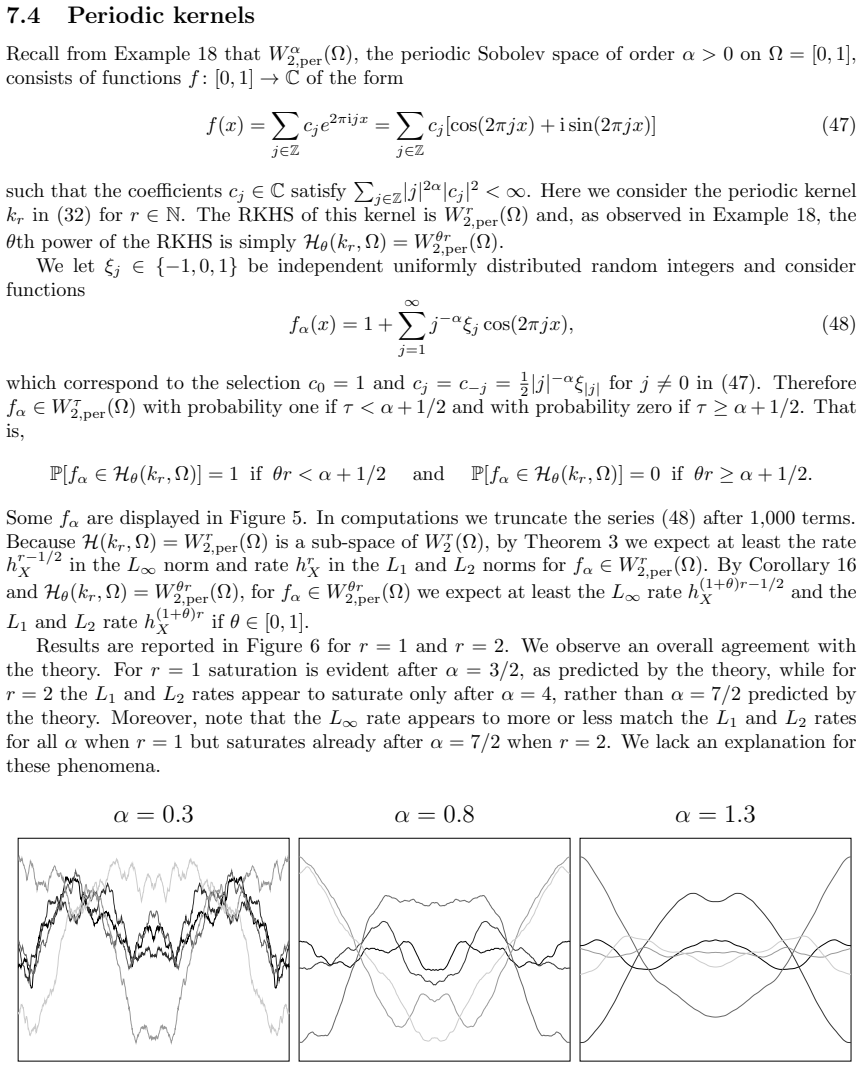
- [Section 7.4, Eq. (48)] The statement that f_α(x)=1+Σ_{j≥1} j^{-α} ξ_j cos(2πjx) lies in W^τ_{2,per}(Ω) with probability one iff τ < α+1/2 is false. The Fourier coefficients decay as |c_j| ≍ j^{-α}, so E∥f_α∥^2_{W^τ_{2,per}} ≍ Σ_{j≥1} j^{2τ-2α}, which converges exactly when τ < α−1/2; by the three-series theorem the same threshold holds almost surely. Consequently, all membership predictions for H^θ(k_r,Ω) in the discussion of Figure 6 are shifted by one full derivative. In particular, the reported anomaly for r=2 (saturation of the L1 and L2 rates at α=4 instead of the predicted α=7/2) is not a genuine unexplained phenomenon: with the corrected smoothness, the prediction for the h^4-rate saturation moves to α>9/2, which is consistent with the observation that saturation occurs later than 7/2. The claimed 'agreement with theory' for r=1 is likewise not established as stated. Section 7.4 and the related comments in Section 8 must be re-evaluated with the corrected threshold.
- [Corollary 10, Eq. (23)] The displayed bound ∥v−Pv∥_H ≤ ∥v∥_{(H,A*(V'))_{θ,∞}} ε^θ omits a factor 2 that appears in the proof. The proof yields ∥v−Pv∥_H ≤ 2K(ε,v) ≤ 2∥v∥_{(H,A*(V'))_{θ,∞}} ε^θ. The statement should include this factor, and the same constant should be tracked in the subsequent corollaries (or the text should note explicitly that constants are ignored). As written, the corollary states a stronger inequality than the proof establishes.
minor comments (6)
- [Section 2.4, Theorem 4] The bound is stated with ∥v∥_{L2(Ω)} on the right-hand side, but the standard argument via identity (13) gives ∥g∥_{L2(Ω)} for v=Tg, i.e., the T(L2)-norm of v. Please verify the exact statement in [37] and in Theorem 11.23 of [42]; if the L2 norm is intended, explain how it is obtained, and otherwise correct Theorem 4 and Corollary 5 accordingly.
- [Section 5, first paragraph] There is a typo: 'In thi section' should read 'In this section'.
- [Figure 1] The label 'TL 1(Ω)' is ambiguous; it should be typeset as T(L^1(Ω)) to avoid confusion with a product or a new space name.
- [Section 7.1] For integer α, the function x^α is a polynomial and therefore belongs to W^σ_2(Ω) for every σ; the statement 'except for integer values of α, the Sobolev smoothness of f_α scales according to α' is imprecise and should be qualified.
- [Section 7.4] The text reports saturation thresholds using the parameter α, while Figure 6 labels the horizontal axis as 'Smoothness α+1/2'. Please state explicitly whether statements such as 'after α = 3/2' refer to the exponent α or to the smoothness value α+1/2, to avoid an apparent mismatch with the figure.
- [Section 8] The sentence referring to 'a saturation of these rates to values that are larger than predicted by a 1/2 term' is vague and depends on the miscalibrated Section 7.4; it should be rewritten after correcting the periodic experiment.
Circularity Check
No significant circularity: the derivation is self-contained and the bounds follow from standard adjoint/interpolation arguments; the Section 7.4 threshold error is a correctness issue, not a circular step.
full rationale
The central results are not circular. Theorem 6 is a direct adjoint calculation: from (15), ∥A(f−Pf)∥_V ≤ ε∥f∥_H, and v=A*g, the paper obtains |⟨v,f−Pf⟩_H|=|g(A(f−Pf))| ≤ ‖g‖_{V′} ε‖f‖_H, giving (16). No part of the conclusion is used as an assumption. Corollary 10 is a standard real-interpolation argument using the K-functional, and Corollary 15/16 merely combine that interpolation bound with the external scattered-data estimate of Theorem 3. The power-space constructions in Section 4 are explicitly characterized via Mercer eigenvalues, and Lemma 14 is proved from a cited interpolation theorem; the boundary-condition discussion in Section 6 is supported by Green-kernel/PDE results rather than by fitting. The numerical experiments compare independently estimated slopes to the stated rates; they do not set free parameters to force those rates. The only self-citations are contextual: [30] is used to reformulate Example 12 and [44] is cited for inverse statements in the misspecified setting, neither of which is load-bearing for the superconvergence theorem. The one substantive concern is not circularity: Section 7.4 states that f_α in (48) lies in W^τ_{2,per} iff τ < α+1/2, whereas the Fourier-coefficient threshold is τ < α−1/2. This miscalibration explains the 'unexplained' saturation discrepancies in Figure 6 and weakens the experimental validation, but it does not feed back into the proof of Theorem 6 or Corollary 16.
Assumptions & free parameters
assumptions (5)
- domain assumption Mercer's theorem conditions (Assumption 1): the kernel integral operator T has a countable orthonormal eigenbasis of L2(Ω) and {λ_j^{1/2}φ_j} is an ONB of H(Ω).
- domain assumption Sobolev fill-distance error bound (Theorem 3): for a Sobolev kernel of order τ on a bounded Lipschitz domain satisfying an interior cone condition, |f−I_X f|_{W_q^m} ≤ C h^{τ−m−d(1/2−1/q)_+} ∥f−I_X f∥_H.
- domain assumption Spectral summability bound: sup_{x∈Ω} Σ_j λ_j^{2−θ} φ_j(x)^2 ≤ κ^2 whenever (2−θ)τ > d/2.
- standard math Real interpolation theory for Hilbert spaces (Chandler-Wilde et al. [4], Lunardi [20]).
- domain assumption Green kernel/PDE representation of adjoint embeddings for Sobolev spaces (Hubmer-Sherina-Ramlau [11], Saitoh et al. [28]).
Cite this review
Pith. "Pith review of General superconvergence for kernel-based approximation." pith.science (2026). https://pith.science/paper/MYBYWOBR
@misc{pith2026250511435,
  author       = {Pith},
  title        = {Pith review of: General superconvergence for kernel-based approximation},
  year         = {2026},
  howpublished = {\url{https://pith.science/paper/MYBYWOBR}},
  note         = {Machine review of arXiv:2505.11435}
}
abstract
Kernel interpolation is a fundamental technique for approximating functions from scattered data, with a well-understood convergence theory when interpolating elements of a reproducing kernel Hilbert space. Beyond this classical setting, research has focused on two regimes: misspecified interpolation, where the kernel smoothness exceeds that of the target function, and superconvergence, where the target is smoother than the Hilbert space. This work addresses the latter, where smoother target functions yield improved convergence rates, and extends existing results by characterizing superconvergence for projections in general Hilbert spaces. We show that functions lying in ranges of certain operators, including adjoint of embeddings, exhibit accelerated convergence, which we extend across interpolation scales between these ranges and the full Hilbert space. In particular, we analyze Mercer operators and embeddings into $L_p$ spaces, linking the images of adjoint operators to Mercer power spaces. Applications to Sobolev spaces are discussed in detail, highlighting how superconvergence depends critically on boundary conditions. Our findings generalize and refine previous results, offering a broader framework for understanding and exploiting superconvergence. The results are supported by numerical experiments.
Figures


Figures from the paper (3 more)


Forward citations
Cited by 3 Pith papers
-
Divergence-free interpolation of tangential vector fields via matrix-valued kernels
A new class of surface divergence-free kernel interpolants preserves the scalar kernel's Sobolev order with m=1 and adds a multiplier-preserving inverse Laplace-Beltrami variant.
-
Do Neural Networks Really Beat the Curse of Dimensionality? A Bit-Complexity View
When approximation quality is measured per bit instead of per parameter, neural networks do not fundamentally beat classical methods; the real limit is the metric entropy of the target function class.
-
Piecewise linear interpolation via kernels
Piecewise linear spline interpolation is kernel interpolation with kernels that are Green functions of a second-order boundary-value problem, and kernel superconvergence reproduces the classical linear-spline rates.
Reference graph
Works this paper leans on
-
[1]
P. Acquistapace and B. Terreni. H¨ older classes with boundary conditions as interpolation spaces. Mathematische Zeitschrift, 195(4):451–471, 1987
work page 1987
-
[2]
A. Berlinet and C. Thomas-Agnan. Reproducing Kernel Hilbert Spaces in Probability and Statistics. Springer, 2004
work page 2004
-
[3]
G. Blanchard and N. M¨ ucke. Optimal rates for regularization of statistical inverse learning problems. Foundations of Computational Mathematics , 18(4):971–1013, 2018. 26
work page 2018
-
[4]
S. N. Chandler-Wilde, D. P. Hewett, and A. Moiola. Interpolation of Hilbert and Sobolev spaces: quantitative estimates and counterexamples. Mathematika, 61(2):414–443, 2015
work page 2015
-
[5]
G. E. Fasshauer. Green’s functions: Taking another look at kernel approximation, radial basis functions, and splines. In Approximation theory XIII: San Antonio 2010 , volume 13 of Springer Proceedings in Mathematics, pages 37–63. Springer, 2012
work page 2010
-
[6]
G. E. Fasshauer and M. J. McCourt. Kernel-based Approximation Methods using MATLAB , volume 19. World Scientific Publishing Company, 2015
work page 2015
-
[7]
G. E. Fasshauer and Q. Ye. Reproducing kernels of generalized Sobolev spaces via a Green function approach with distributional operators. Numerische Mathematik, 119:585–611, 2011
work page 2011
-
[8]
G. E. Fasshauer and Q. Ye. Reproducing kernels of Sobolev spaces via a Green kernel approach with differential operators and boundary operators. Advances in Computational Mathematics, 38:891–921, 2013
work page 2013
Show all 46 references
-
[9]
Fischer and I
S. Fischer and I. Steinwart. Sobolev norm learning rates for regularized least-squares algo- rithms. Journal of Machine Learning Research , 21(205):1–38, 2020
2020
-
[10]
Hangelbroek and C
T. Hangelbroek and C. Rieger. Extending error bounds for radial basis function interpola- tion to measuring the error in higher order Sobolev norms. Mathematics of Computation , 94(351):381–407, 2025
2025
-
[11]
Hubmer, E
S. Hubmer, E. Sherina, and R. Ramlau. Characterizations of adjoint sobolev embedding operators with applications in inverse problems. Electron. Trans. Numer. Anal., 59:116–144, 2023
2023
-
[12]
A. Iske. Approximation Theory and Algorithms for Data Analysis , volume 68 of Texts in Applied Mathematics. Springer, Cham, 2018
2018
-
[13]
M. J. Johnson. On the error in surface spline interpolation of a compactly supported function. Kuwait Journal of Science and Engineering , 28(1):37–54, 2001
2001
-
[14]
Kanagawa, B
M. Kanagawa, B. K. Sriperumbudur, and K. Fukumizu. Convergence guarantees for kernel- based quadrature rules in misspecified settings. In Advances in Neural Information Processing Systems, volume 29, pages 3288–3296, 2016
2016
-
[15]
Kanagawa, B
M. Kanagawa, B. K. Sriperumbudur, and K. Fukumizu. Convergence analysis of determin- istic kernel-based quadrature rules in misspecified settings. Foundations of Computational Mathematics, 20(1):155–194, 2020
2020
-
[16]
Karvonen
T. Karvonen. Error bounds and the asymptotic setting in kernel-based approximation. Dolomites Research Notes on Approximation , 15:65–77, 2022
2022
-
[17]
Li and J
Y. Li and J. W. Siegel. Entropy-based convergence rates of greedy algorithms. Mathematical Models and Methods in Applied Sciences , 34(05):779–802, 2024
2024
-
[18]
Y. Li, H. Zhang, and Q. Lin. On the saturation effect of kernel ridge regression. arXiv:2405.09362, 2024
2024 arXiv
-
[19]
L¨ ohndorf and J
M. L¨ ohndorf and J. M. Melenk. On thin plate spline interpolation. In Spectral and High Order Methods for Partial Differential Equations ICOSAHOM 2016: Selected Papers from the ICOSAHOM conference, June 27-July 1, 2016, Rio de Janeiro, Brazil , pages 451–466. Springer, 2017
2016
-
[20]
A. Lunardi. Interpolation Theory, volume 16 of Publications of the Scuola Normale Superiore . Springer, 2018
2018
-
[21]
Mohebalizadeh, G
H. Mohebalizadeh, G. E. Fasshauer, and H. Adibi. Refined error estimates for Green kernel- based interpolation. Applied Mathematics Letters, 133:108258, 2022. 27
2022
-
[22]
Musina and A
R. Musina and A. I. Nazarov. On fractional Laplacians – 2. Annales de l’Institut Henri Poincar´ e C, Analyse non lin´ eaire, 33(6):1667–1673, 2016
2016
-
[23]
F. J. Narcowich, J. D. Ward, and H. Wendland. Sobolev bounds on functions with scattered zeros, with applications to radial basis function surface fitting. Mathematics of Computation , 74(250):743–763, 2005
2005
-
[24]
F. J. Narcowich, J. D. Ward, and H. Wendland. Sobolev error estimates and a Bernstein inequality for scattered data interpolation via radial basis functions. Constructive Approxi- mation, 24(2):175–186, Sep 2006
2006
-
[25]
Novak and H
E. Novak and H. Wo´ zniakowski. Tractability of Multivariate Problems. Volume I: Linear Information, volume 6 of EMS Tracts in Mathematics. European Mathematical Society, 2008
2008
-
[26]
V. I. Paulsen and M. Raghupathi. An Introduction to the Theory of Reproducing Kernel Hilbert Spaces, volume 152 of Cambridge Studies in Advanced Mathematics . Cambridge University Press, 2016
2016
-
[27]
Porcu, M
E. Porcu, M. Bevilacqua, R. Schaback, and C. J. Oates. The Mat´ ern model: A journey through statistics, numerical analysis and machine learning. Statistical Science, 39(3):469–492, Aug 2024
2024
-
[28]
T. Y. S. Saitoh, K. Watanabe and W. Takahashi. Reproducing kernels ofHm(a,b ) (m = 1, 2, 3) and least constants in Sobolev’s inequalities. Applicable Analysis, 82(8):809–820, 2003
2003
-
[29]
Saitoh and Y
S. Saitoh and Y. Sawano. Theory of Reproducing Kernels and Applications , volume 44 of Developments in Mathematics . Springer, 2016
2016
-
[30]
Santin, T
G. Santin, T. Karvonen, and B. Haasdonk. Sampling based approximation of linear functionals in reproducing kernel Hilbert spaces. BIT Numerical Mathematics , 62:279–310, 2021
2021
-
[31]
Schaback
R. Schaback. Error estimates and condition numbers for radial basis function interpolation. Advances in Computational Mathematics , 3(3):251–264, 1995
1995
-
[32]
Schaback
R. Schaback. Improved error bounds for scattered data interpolation by radial basis functions. Mathematics of Computation , 68(225):201–216, 1999
1999
-
[33]
Schaback
R. Schaback. Superconvergence of kernel-based interpolation. Journal of Approximation Theory, 235:1–19, 2018
2018
-
[34]
Schaback
R. Schaback. Small errors imply large evaluation instabilities. Advances in Computational Mathematics, 49(2):25, 2023
2023
-
[35]
Schaback and H
R. Schaback and H. Wendland. Approximation by positive definite kernels. In Advanced Prob- lems in Constructive Approximation: 3rd International Dortmund Meeting on Approximation Theory (IDoMAT) 2001, pages 203–222. Springer, 2002
2001
-
[36]
Sch¨ olpple and I
M. Sch¨ olpple and I. Steinwart. Which spaces can be embedded in Reproducing Kernel Hilbert Spaces? Constructive Approximation, 2025
2025
-
[37]
I. H. Sloan and V. Kaarnioja. Doubling the rate: improved error bounds for orthogonal projection with application to interpolation. BIT Numerical Mathematics , 65(1):10, 2025
2025
-
[38]
B. K. Sriperumbudur, K. Fukumizu, and G. R. G. Lanckriet. Universality, characteristic kernels and rkhs embedding of measures. J. Mach. Learn. Res. , 12:2389–2410, 2011
2011
-
[39]
Steinwart
I. Steinwart. Convergence types and rates in generic Karhunen-Lo` eve expansions with appli- cations to sample path properties. Potential Analysis, 51:361–395, 2019
2019
-
[40]
Steinwart and C
I. Steinwart and C. Scovel. Mercer’s theorem on general domains: On the interaction between measures, kernels, and RKHSs. Constructive Approximation, 35:363–417, 2012. 28
2012
-
[41]
Wendland
H. Wendland. Piecewise polynomial, positive definite and compactly supported radial func- tions of minimal degree. Advances in Computational Mathematics , 4(1):389–396, 1995
1995
-
[42]
Wendland
H. Wendland. Scattered Data Approximation, volume 17 of Cambridge Monographs on Applied and Computational Mathematics . Cambridge University Press, 2005
2005
-
[43]
Wendland and J
H. Wendland and J. K¨ unemund. Solving partial differential equations on (evolving) surfaces with radial basis functions. Advances in Computational Mathematics , 46(4):64, 2020
2020
-
[44]
T. Wenzel. Sharp inverse statements for kernel interpolation. Mathematics of Computation , 2025
2025
-
[45]
Wenzel, G
T. Wenzel, G. Santin, and B. Haasdonk. Analysis of target data-dependent greedy kernel algorithms: Convergence rates for f-, f · P -and f/P -greedy. Constructive Approximation , 57(1):45–74, 2023
2023
-
[46]
Wenzel, D
T. Wenzel, D. Winkle, G. Santin, and B. Haasdonk. Adaptive meshfree solution of linear partial differential equations with PDE-greedy kernel methods. BIT Numerical Mathematics, 65(11), 2025. 29
2025
Reviewed August 15, 2026 · model on record in the stance chip above.
Discussion (0). Continue with ORCID to comment.