Combined Tail Estimation Using Censored Data and Expert Information

Hansjoerg Albrecher; Jan Beirlant; Martin Bladt

REVIEW 3 major objections 4 minor 15 references

Combined Tail Estimation Using Censored Data and Expert Information

T0 review · 3 major / 4 minor · reviewed 2026-08-14 · deepseek-v4-flash

Challenge this review Re-run · record.json Download PDF Read on arXiv ↗ Review JSON

Pith's one-line read This paper claims that an entropy-penalized likelihood can blend the censored Hill estimator with expert tail-index guesses, and that with a correct expert guess the blend is asymptotically normal and has lower variance than censored Hill…

desk verdict A genuinely useful censored-tail estimator with an explicit expert combination formula, though the λ=1 rule leans on a clairvoyant expert and no safeguard is offered. read the letter →

arxiv 1908.03390 v2 pith:N45BXULU submitted 2019-08-09 stat.AP stat.ME

Martin Bladt , Hansjoerg Albrecher , Jan Beirlant This is my paper · ORCID

classification stat.APstat.ME MSC 62G3262N0162P05

keywords tailindexestimationrandomcensoringexpertinformationentropy-perturbedlikelihoodHillestimatorregularvariationextremevaluestatisticsliabilityinsurance

verification ladder T0 review T1 audit T2 compute T3 formal

The pith

A machine-rendered reading of the paper's core claim, the machinery that carries it, and where it could break.

The reading

In liability insurance, claim sizes are often right-censored because claims stay open for years, but experts maintain projections for those open claims. This paper proposes using that expert information in heavy-tail estimation by adding an entropy-based penalty to the Pareto-type likelihood. Its main result is that for penalty strength $\lambda=1$ the reciprocal of the new estimator is exactly a weighted average of the reciprocal of the censored Hill estimator and $1/\beta$, with weights the observed proportions of uncensored and censored observations among the largest $k$ claims. Under the Hall second-order condition and a correct expert guess ($\beta=\alpha$) the reciprocal of the estimator is asymptotically normal with variance $1/[kp(\alpha+\alpha_2)^2]$, smaller than the censored Hill estimator's variance. The paper thereby offers a parameter-free way to combine closed-claim data with expert judgment, and a simulation study plus a motor third-party liability insurance dataset show it often beats censored Hill and two Bayesian benchmarks.

What carries the argument

The engine is the entropy-perturbed likelihood: multiply the usual censored Pareto likelihood by $e^{-\lambda(1-e_i)D(\alpha,\beta_i)}$, where $D$ is the Kullback-Leibler divergence between a Pareto density with tail index $\alpha$ and the expert's Pareto density with tail index $\beta_i$. That specific divergence makes the maximizer explicit, turns the penalty into a gamma-type prior whose strength is governed by the censoring indicators, and at $\lambda=1$ collapses to the weighted-average identity in Corollary 4.4. The asymptotic results then flow from the Hall-class expansion of the censored tail quantile function and from the known joint limit behaviour of the Hill statistic and the censoring proportion.

What would settle it

Simulate from a known Hall-class model with tail index $\alpha$ and censoring tail index $\alpha_2$, feed the estimator the true value $\beta=\alpha$ and $\lambda=1$, and check the empirical variance of the reciprocal estimator against $1/[kp(\alpha+\alpha_2)^2]$ for large $k$; if the realized variance does not fall below the censored Hill variance $1/(kp\alpha^2)$, Corollary 4.4 is not confirmed.

Watch

Extended reading notes

Core claim

Working with exact Pareto distributions first, the authors perturb the censored-data likelihood by a factor $e^{-\lambda(1-e_i)D(\alpha,\beta_i)}$ with $D$ the Kullback-Leibler divergence between Pareto densities, so the log-likelihood becomes $\sum_i e_i\log f_\alpha(Z_i)+\sum_i(1-e_i)\log\bar F_\alpha(Z_i)-\lambda\sum_i(1-e_i)D(\alpha,\beta_i)$. The maximizer is explicit: $\hat\alpha^P(\lambda)=\sum_i(e_i+\lambda(1-e_i))/\sum_i(\log(Z_i/x_0)+\lambda(1-e_i)/\beta_i)$, which reduces to the censored Hill estimator as $\lambda\to0$ and to the experts' harmonic mean as $\lambda\to\infty$. For Pareto-type tails in the Hall class, Theorem 4.1 establishes asymptotic normality of the reciprocal estimator, and Corollary 4.4 shows that when $\lambda=1$, the second-order bias vanishes ($\delta=0$), and the expert guesses equal the true index ($\beta=\alpha$), one has $1/\hat\alpha^P_k=\hat p_k/\hat\alpha^{MLE}_k+(1-\hat p_k)/\beta$; that is, the inverse estimate is the censoring-weighted average of the inverse censored-Hill estimate and the inverse expert tail index. Its asymptotic variance is $1/[kp(\alpha+\alpha_2)^2]$, improving on the censored Hill benchmark. The same combination is used to define a quantile estimator, and simulations plus an MTPL insurance case study support the method.

Load-bearing premise

The load-bearing premise is that the expert's tail-index guess $\beta$ is actually right, because the clean unbiasedness and variance reduction only hold for $\beta=\alpha$; with a biased or uninformative guess, the $\lambda=1$ estimator can be more biased than the censored Hill estimator that ignores the expert entirely.

Editorial extensions

If this is right

With a reliable expert guess, the estimator replaces tuning by a fixed rule: the reciprocal estimate is $\hat p_k$ times the reciprocal censored-Hill estimate plus $(1-\hat p_k)/\beta$, so the data weight is exactly the observed fraction of uncensored observations among the largest $k$ claims.
In Hall-class models with a clairvoyant expert, the asymptotic variance of the reciprocal estimator is $1/[kp(\alpha+\alpha_2)^2]$, strictly smaller than the censored Hill variance $1/(kp\alpha^2)$, and the reduction grows as the censoring tail becomes heavier.
The same weighted-average rule carries over to quantile estimation: the combined high quantile is a weighted geometric combination of the Kaplan-Meier based extrapolation and the expert-based extrapolation, yielding a stable compromise between the two.
As $\lambda\to0$ the estimator collapses to the censored Hill estimator and as $\lambda\to\infty$ it collapses to the expert's harmonic mean, so the method forms a continuum with the proposed $\lambda=1$ as a natural no-tuning choice.
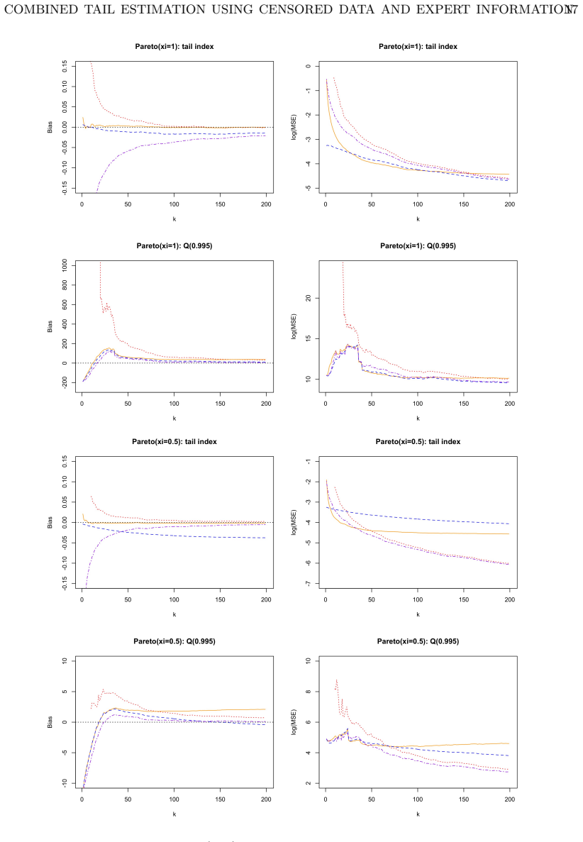
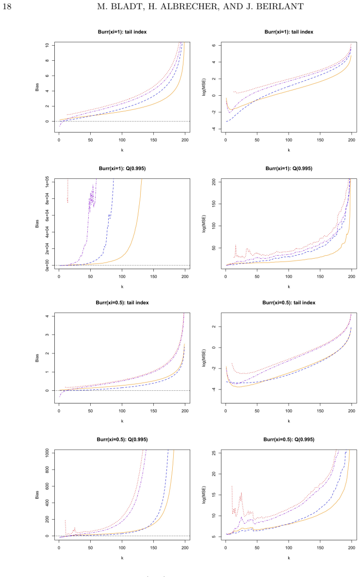
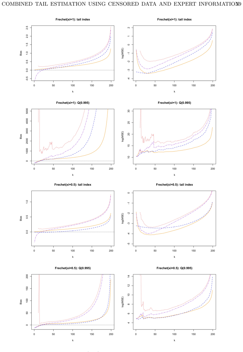
In the paper's simulations across Pareto, Burr, and Fréchet tails, the combined estimator frequently has lower bias and MSE than censored Hill and the two Bayesian benchmarks, especially for heavy tails and for quantiles under non-Pareto tails.

Reading between the lines

Editorial extensions of the paper, not claims the author makes directly.

Because the variance ratio is $\alpha^2/(\alpha+\alpha_2)^2$, the largest gains from expert information occur exactly in the high-censoring regime that motivates the paper; a natural test would be to measure the estimator's advantage as a function of the censoring fraction.
The same entropy-penalty mechanism could replace the censored Hill baseline with bias-reduced or trimmed Hill estimators inside the combination formula, which the paper flags as future work on trimming.
The Bayesian reading suggests an explicit hierarchical extension: treat each expert $\beta_i$ as a draw from a prior with its own uncertainty and let $\lambda$ control the prior's weight, which would yield a diagnostic for when expert information is too noisy to use.
Since the paper gives no data-driven way to choose $\lambda$, a practical extension is to select $\lambda$ by the stability of $\hat\alpha^P_k$ across thresholds $k$, or by comparing it with the censored Hill estimator to detect expert bias.

Share X Bluesky LinkedIn Reddit HN

Signed reviews

No signed human review yet.

Editorial analysis

A structured set of objections, weighed in public.

Desk editor's note, referee report, and a circularity audit.

Desk Editor's Note

read the letter

The real new thing here is the entropy-perturbed likelihood estimator for Pareto-type tails with random censoring and expert guesses on the tail index. It is not a repackaged Hill estimator: the explicit formula, the asymptotic normality under Hall-class assumptions, and especially Corollary 4.4's combination identity are original and cleanly derived. The Bayesian-prior analogy is a nice interpretive bonus, and the paper is honest that it is not a true Bayesian method.

The derivations hold up. I checked Theorem 4.1's algebra in outline; the variance and bias expressions are plausible and the cancellation that kills the r2 term is real. The proof sketch in the appendix is thin in places but the ingredients are standard, and the omitted algebra is routine. The simulation study is fair to the competitors: the Bayesian gamma estimator is given extra information (true variance) while the proposed estimator uses only λ=1, and the new estimator still wins often. That is real evidence.

The soft spot is exactly what the stress-test note says: the λ=1 rule is justified only when β=α and second-order bias δ=0. With any fixed misspecification β≠α, the combined estimator has a permanent asymptotic bias (1−p)(1/β−1/α) and is inconsistent, while censored Hill stays consistent. So the variance reduction advertised in Corollary 4.4 is local to a clairvoyant expert. The paper acknowledges the dependence on expert quality in Section 5 but offers no diagnostic or data-driven safeguard; Remark 5.1 dismisses cross-validation for good reasons, but that leaves practitioners with no way to check whether the expert guess is in the right ballpark. Also, the case study uses β derived from the same dataset's ultimates, which cannot validate the independence of the expert information. These are addressable issues: a sensitivity analysis with biased experts, or a data-driven check on β, would materially strengthen the paper.

Overall, this is a solid methodological contribution for actuarial heavy-tail estimation. The central estimator is useful, the math is sound under stated assumptions, and the limitations are honestly disclosed. A serious referee should engage with it. I would not desk-reject, and I would cite it if I worked on censored extremes.

Referee Report

3 major / 4 minor

Summary. The manuscript proposes a penalized-likelihood estimator for the tail index of Pareto-type data under random right censoring, where each censored observation is accompanied by an expert-supplied tail index. The penalty is the relative entropy between Pareto densities, which yields an explicit estimator of Hill type that interpolates between the censored maximum-likelihood (Hill) estimator and the expert information as the penalization strength λ varies. Section 3 gives a Bayesian/gamma-prior interpretation, Section 4 derives asymptotic normality under the Hall class, and Corollary 4.4 shows that for λ = 1, β = α, and δ = 0, the reciprocal estimator is a weighted average of the censored Hill estimator and the expert tail index, with asymptotic variance 1/[kp(α + α2)^2]. Section 5 reports simulations against censored Hill and two Bayesian estimators, and applies the method to motor third-party liability insurance claims.

Significance. If the main claims hold, the paper provides a simple, explicit, and interpretable rule for combining expert tail information with censored data, together with a Bayesian analogy and a quantile extension. The derivations in Section 2 and Appendix A are largely explicit, and the asymptotic variance formula in Theorem 4.1 is a useful technical contribution. However, the advertised variance reduction and the λ = 1 recommendation are proven only under a clairvoyant expert condition (β = α) and a vanishing second-order bias condition (δ = 0), which the paper itself acknowledges only in passing. The simulation evidence conditions on expert guesses that are centered at the true value, and the case study derives β from the same dataset, so the empirical support is weaker than the wording suggests. The contribution is therefore valuable as a conditional combination tool, but the paper needs to address misspecification and provide safeguards before the practical recommendation can be accepted.

major comments (3)

[§4, Theorem 4.1 and Corollary 4.4] The centering in Theorem 4.1 shows that for λ = 1 and δ = 0 the probability limit of 1/α̂^P_k is (1 + α2/β)/(α + α2) = p/α + (1 − p)/β, which equals 1/α only when β = α. For any fixed expert misspecification β ≠ α, the estimator 1/α̂^P_k has permanent asymptotic bias (1 − p)(1/β − 1/α), so its AMSE tends to a positive constant while the censored Hill estimator remains consistent. The variance reduction claimed in Corollary 4.4 therefore holds only in the clairvoyant case, and the paper does not provide an analysis of the bias–variance trade-off for misspecified experts. I would ask the authors to add an explicit misspecification analysis, at least for the Hall class with δ = 0, and to temper or qualify the recommendation of λ = 1 accordingly.
[§5.1, simulation design] The simulations generate the expert input by drawing a single random number from a Gaussian distribution centered at the true ξ with standard deviation 0.2, and the Bayesian competitor is given the true variance by moment matching. This makes the comparison favorable by construction. The text in §5.1 concedes that changed conditions can make both the perturbed and Bayesian estimators perform much worse, but no such scenario is reported. Since the central empirical claim is that the estimator 'often outperforms' the benchmarks, the paper should include misspecified-expert scenarios, such as β drawn from a distribution with a nonzero mean shift or larger variance, and report bias and MSE relative to the censored Hill estimator.
[§5, Remark 5.1 and §6] The paper rejects cross-validation for selecting λ in Remark 5.1 but offers no alternative data-driven safeguard, and the conclusion reiterates that no tuning parameter selection is needed. Given that λ = 1 is only formally justified when β = α and δ = 0, the practical recommendation is incomplete: a practitioner with an uncertain expert guess has no guidance on when the combined estimator is preferable to censored Hill. I would ask for at least a diagnostic based on the discrepancy between the expert value and the censored-Hill estimate, or a clear statement identifying the conditions under which λ = 1 is safe to use.

minor comments (4)

[§5.1] The text refers to the 'Weismann estimator'; the correct spelling is Weissman, as in the references.
[§5.2 and §6] The references to 'Theorem 4.4' should refer to Corollary 4.4, which is the statement being used.
[§4, Eq. (29)] The final expression in Eq. (29) uses \\hat\\xi^P_k, but that notation is only introduced later in Eq. (31); please define \\hat\\xi^P_k before the quantile formula.
[§4, Corollary 4.4] The statement that the estimator is 'unbiased' should explicitly say 'asymptotically unbiased under the conditions β = α and δ = 0', since the unbiasedness is not a finite-sample property and depends on the clairvoyance assumption.

Circularity Check

0 steps flagged · score 0.0 of 10

No significant circularity: the combined estimator is derived from a penalized likelihood with external expert inputs, and the λ=1 combination formula is algebra, not an input.

full rationale

The central derivation (Theorem 4.1, Corollary 4.4) starts from the entropy-perturbed likelihood (5) with explicit minimizer α̂^P_k. Corollary 4.4's identity, 1/α̂^P_k = p̂_k(1/α̂^MLE_k)+(1-p̂_k)/β for λ=1, follows by direct algebra from the definitions of H_k, p̂_k and α̂^MLE_k; it is not assumed as an input. The expert index β is an external quantity supplied before estimation, not fitted to the data used to evaluate the estimator, and the variance comparison assumes β=α explicitly, which is a stated condition rather than a hidden circularity. Citations [2], [3], [8], [10] provide standard asymptotic and Hill-estimator results; [15] supplies the case-study value ξ=0.48 for the ultimates, but this affects only the illustrative application and is disclosed ('we know how β is obtained'). The simulation generates expert guesses from N(ξ,0.2), which is a study design for investigating behavior under expert error, not a circular validation. No fitted parameter is renamed as a prediction, and no load-bearing premise is justified solely by self-citation. The principal limitations (bias under β≠α, no safeguard) are correctness/robustness concerns, not circularity.

Assumptions & free parameters 2 free parameters · 5 assumptions · 0 invented entities

The method introduces no new physical or conceptual entities. It adds two inputs beyond the raw censored data: a scalar penalty λ and expert tail indices β_i, the latter being an external belief rather than an estimated parameter. The main assumptions are the standard EVT Hall class and random censoring, plus the paper-specific choices of KL-divergence penalization and the idealized clairvoyant condition used for the clean theorem.

free parameters (2)

penalization strength λ = recommended 1, otherwise user-chosen
Controls the weight placed on expert information relative to the data; set to 1 in Corollary 4.4 to obtain the simple combination formula, with optimality proven only in the clairvoyant case.
expert tail index β = 1/0.48 in the MTPL case study; drawn as 1/(N(ξ, 0.2)) in simulations.
External input representing the expert's belief about the tail; the estimator's performance depends on its accuracy, and in the case study it is estimated from the same dataset's ultimates.

assumptions (5)

domain assumption The claim data follow a Pareto-type distribution in the Hall class with second-order regular variation (equation 15).
Standard EVT condition used in Section 4 to derive asymptotic normality; if the Hall class fails, the bias terms in Theorem 4.1 do not have the stated form.
domain assumption Censoring is random: Z_i = min(X_i, L_i) with X_i and L_i independent, both with regularly varying tails.
Defines the censoring mechanism in Section 4 and determines the limiting proportion of censored observations p; if censoring depends on claim size, the estimator's variance formula changes.
domain assumption Every observation shares a common tail index α, and each censored observation carries an expert tail parameter β_i that is informative about α.
The entire construction rests on this premise (Section 1); the paper acknowledges that bad expert guesses make the method worse than ignoring them.
ad hoc to paper The relative entropy D(α, β_i) in equation (4) is the appropriate dissimilarity measure for penalizing censored contributions.
Remark 2.1 states the choice is mathematical, made so the penalized likelihood has an explicit solution; other divergences yield more complicated estimators.
ad hoc to paper For the clean combination result, the expert is clairvoyant (β = α) and the second-order bias term δ vanishes.
Corollary 4.4 assumes both to obtain unbiasedness and the variance reduction; in practice β is a guess and δ is rarely zero.

how reviews work

0 comments

Cite this review

Pith. "Pith review of Combined Tail Estimation Using Censored Data and Expert Information." pith.science (2026). https://pith.science/paper/N45BXULU

@misc{pith2026190803390,
  author       = {Pith},
  title        = {Pith review of: Combined Tail Estimation Using Censored Data and Expert Information},
  year         = {2026},
  howpublished = {\url{https://pith.science/paper/N45BXULU}},
  note         = {Machine review of arXiv:1908.03390}
}

read the original abstract

We study tail estimation in Pareto-like settings for datasets with a high percentage of randomly right-censored data, and where some expert information on the tail index is available for the censored observations. This setting arises for instance naturally for liability insurance claims, where actuarial experts build reserves based on the specificity of each open claim, which can be used to improve the estimation based on the already available data points from closed claims. Through an entropy-perturbed likelihood we derive an explicit estimator and establish a close analogy with Bayesian methods. Embedded in an extreme value approach, asymptotic normality of the estimator is shown, and when the expert is clair-voyant, a simple combination formula can be deduced, bridging the classical statistical approach with the expert information. Following the aforementioned combination formula, a combination of quantile estimators can be naturally defined. In a simulation study, the estimator is shown to often outperform the Hill estimator for censored observations and recent Bayesian solutions, some of which require more information than usually available. Finally we perform a case study on a motor third-party liability insurance claim dataset, where Hill-type and quantile plots incorporate ultimate values into the estimation procedure in an intuitive manner.

Figures

Figures reproduced from arXiv: 1908.03390 by the authors.

**Figure 1.** Motor third-party liability insurance: log-claims in vertical order of arrival, showing the paid amount for both open (red, circle) and closed (black, dot) claims, as well as ultimate values for the open claims (green, triangle). as well as the Hill estimator for heavy and Pareto-like tails. This research has started in [2] and [3] and has received more attention recently, see e.g. [4], [5], [6]. However, in that li… view at source ↗

**Figure 2.** Bias and (log) Mean Square Error for the exact Pareto distribution, for varying parameters. We compare ˆξ P k (orange, solid), ˆξ MLE k (red, dotted), ˆξ BG k (blue, dashed) and ˆξ BM k (purple, dashed and dotted), as well as the associated Weissman quantile estimator [PITH_FULL_IMAGE:figures/full_fig_p017_2.png] view at source ↗

**Figure 3.** Bias and (log) Mean Square Error for the Burr distribution, for varying parameters. We compare ˆξ P k (orange, solid), ˆξ MLE k (red, dotted), ˆξ BG k (blue, dashed) and ˆξ BM k (purple, dashed and dotted), as well as the associated Weissman quantile estimator [PITH_FULL_IMAGE:figures/full_fig_p018_3.png] view at source ↗

Figures from the paper (6 more)

**Figure 4.** Figure 4: Bias and (log) Mean Square Error for the Frechet distribution, for varying parameters. We compare ˆξ P k (orange, solid), ˆξ MLE k (red, dotted), ˆξ BG k (blue, dashed) and ˆξ BM k (purple, dashed and dotted), as well as the associated Weissman quantile estimator [P…

**Figure 5.** Figure 5: Descriptive statistics of the insurance data. Top left: log-claims in order of arrival, showing both open (red, circle) and closed (black, dot) claims. Top right: Kaplan-Meier survival probability estimator for the claims. Bottom left: proportion of closed claims as a…

**Figure 6.** Figure 6: Hill plot of the ultimates (black, dashed), censored Hill estimator ˆξ MLE k for the claims (red, dashed), and the combined estimator ˆξ P k (orange, solid) with λ = 1 and β = 1/0.48. and β = 1/0.48. Notice that in this case, we know how β is obtained, and this additio…

**Figure 7.** Figure 7: Hill plot of the ultimates (black), for the reduced (solid) and complete (dashed) datasets: censored Hill estimator ˆξ MLE k for the claims (red), and the combined estimator ˆξ P k (orange) with λ = 1 and β = 1/0.48 [PITH_FULL_IMAGE:figures/full_fig_p023_7.png]

**Figure 8.** Figure 8: 99.5% quantile estimator using the censored approach (QˆKM k (0.005), red) for the claims, expert information (QˆULT k (0.005), black) and their combination via ˆξ P u , with the selection λ = 1 (QˆP k (0.005), orange) [PITH_FULL_IMAGE:figures/full_fig_p023_8.png]

**Figure 9.** Figure 9: Plot of the 99.5% quantile for the ultimates QˆULT k (black), and for the reduced (solid) and complete (dashed) datasets: censored Hill estimation QˆKM k for the claims (red), and the combined estimator QˆP k (orange) with λ = 1 and β = 1/0.48. the expert is often subj…

Discussion (0). Continue with ORCID to comment.

Reference graph

Works this paper leans on

15 extracted references · 15 canonical work pages

[1]

John Wiley & Sons, 2017

Hansj¨ org Albrecher, Jozef L Teugels, and Jan Beirlant.Reinsurance: Actu- arial and Statistical Aspects . John Wiley & Sons, 2017

work page 2017
[2]

Bias reduced tail estimation for censored pareto type distributions

Jan Beirlant, Goedele Dierckx, Armelle Guillou, and Amelie Fils-Villetard. Bias reduced tail estimation for censored pareto type distributions. Ex- tremes, 10:151–174, 2007

work page 2007
[3]

Statistics of extremes under random censoring

John HJ Einmahl, Am´ elie Fils-Villetard, Armelle Guillou, et al. Statistics of extremes under random censoring. Bernoulli, 14(1):207–227, 2008

work page 2008
[4]

New estimators of the extreme value index under random right censoring, for heavy-tailed distributions

Julien Worms and Rym Worms. New estimators of the extreme value index under random right censoring, for heavy-tailed distributions. Extremes, 17 (2):337–358, 2014

work page 2014
[5]

Bayesian estimation of the tail index of a heavy tailed distribution under random censoring

Abdelkader Ameraoui, Kamal Boukhetala, and Jean-Fran¸ cois Dupuy. Bayesian estimation of the tail index of a heavy tailed distribution under random censoring. Computational Statistics & Data Analysis , 104:148–168, 2016

work page 2016
[6]

Penalized bias reduction in extreme value estimation for censored pareto-type data, and long-tailed insurance applications

Jan Beirlant, Gaonyalelwe Maribe, and Andrehette Verster. Penalized bias reduction in extreme value estimation for censored pareto-type data, and long-tailed insurance applications. Insurance: Mathematics and Economics , 78:114–122, 2018

work page 2018
[7]

Bogaerts, A

K. Bogaerts, A. Komarek, and E. Lesaﬀre. Survival analysis with interval- censored data. Chapman & Hall, Boca Raton, 2018. COMBINED TAIL ESTIMATION USING CENSORED DATA AND EXPERT INFORMATION 27

work page 2018
[8]

A simple general approach to inference about the tail of a distribution

Bruce M Hill. A simple general approach to inference about the tail of a distribution. The Annals of Statistics , 3:1163–1174, 1975

work page 1975

Show all 15 references

[9]

Modelling extremal events: for insurance and ﬁnance , volume 33

Paul Embrechts, Claudia Kl¨ uppelberg, and Thomas Mikosch. Modelling extremal events: for insurance and ﬁnance , volume 33. Springer Science & Business Media, second edition, 2013

2013
[10]

Statistics of Extremes: Theory and Applications

Jan Beirlant, Yuri Goegebeur, Johan Segers, and Jozef Teugels. Statistics of Extremes: Theory and Applications . Wiley, 2004

2004
[11]

Censoring issues in survival analysis

Kwan-Moon Leung, Robert M Elashoﬀ, and Abdelmonem A Aﬁﬁ. Censoring issues in survival analysis. Annual review of public health , 18(1):83–104, 1997

1997
[12]

On some simple estimates of an exponent of regular variation

Peter Hall. On some simple estimates of an exponent of regular variation. J. Roy. Statist. Soc. Ser. B , 44(1):37–42, 1982

1982
[13]

Estimation of parameters and large quantiles based on the k largest observations

Ishay Weissman. Estimation of parameters and large quantiles based on the k largest observations. Journal of the American Statistical Association , 73 (364):812–815, 1978

1978
[14]

E. L. Kaplan and Paul Meier. Nonparametric estimation from incomplete observations. Journal of the American Statistical Association , 53(282):457– 481, 1958

1958
[15]

Trimming and thresh- old selection in extremes

Martin Bladt, Hansjoerg Albrecher, and Jan Beirlant. Trimming and thresh- old selection in extremes. arXiv:1903.07942, 2019. (M. Bladt) Department of Actuarial Science, F aculty of Business and Econom- ics, University of Lausanne, CH-1015 Lausanne, Switzerland E-mail address :...

1903 arXiv

Pith tools

Reviewed August 14, 2026 · model on record in the stance chip above.

[1] [1]

John Wiley & Sons, 2017

Hansj¨ org Albrecher, Jozef L Teugels, and Jan Beirlant.Reinsurance: Actu- arial and Statistical Aspects . John Wiley & Sons, 2017

work page 2017

[2] [2]

Bias reduced tail estimation for censored pareto type distributions

Jan Beirlant, Goedele Dierckx, Armelle Guillou, and Amelie Fils-Villetard. Bias reduced tail estimation for censored pareto type distributions. Ex- tremes, 10:151–174, 2007

work page 2007

[3] [3]

Statistics of extremes under random censoring

John HJ Einmahl, Am´ elie Fils-Villetard, Armelle Guillou, et al. Statistics of extremes under random censoring. Bernoulli, 14(1):207–227, 2008

work page 2008

[4] [4]

New estimators of the extreme value index under random right censoring, for heavy-tailed distributions

Julien Worms and Rym Worms. New estimators of the extreme value index under random right censoring, for heavy-tailed distributions. Extremes, 17 (2):337–358, 2014

work page 2014

[5] [5]

Bayesian estimation of the tail index of a heavy tailed distribution under random censoring

Abdelkader Ameraoui, Kamal Boukhetala, and Jean-Fran¸ cois Dupuy. Bayesian estimation of the tail index of a heavy tailed distribution under random censoring. Computational Statistics & Data Analysis , 104:148–168, 2016

work page 2016

[6] [6]

Penalized bias reduction in extreme value estimation for censored pareto-type data, and long-tailed insurance applications

Jan Beirlant, Gaonyalelwe Maribe, and Andrehette Verster. Penalized bias reduction in extreme value estimation for censored pareto-type data, and long-tailed insurance applications. Insurance: Mathematics and Economics , 78:114–122, 2018

work page 2018

[7] [7]

Bogaerts, A

K. Bogaerts, A. Komarek, and E. Lesaﬀre. Survival analysis with interval- censored data. Chapman & Hall, Boca Raton, 2018. COMBINED TAIL ESTIMATION USING CENSORED DATA AND EXPERT INFORMATION 27

work page 2018

[8] [8]

A simple general approach to inference about the tail of a distribution

Bruce M Hill. A simple general approach to inference about the tail of a distribution. The Annals of Statistics , 3:1163–1174, 1975

work page 1975