Joint elastic full waveform inversion of multi-component geophone and distributed acoustic sensing data
Pith reviewed 2026-07-03 02:26 UTC · model grok-4.3
The pith
A velocity-stress-strain formulation allows direct joint elastic FWI of geophone and DAS data from one forward simulation.
A machine-rendered reading of the paper's core claim, the machinery that carries it, and where it could break.
Core claim
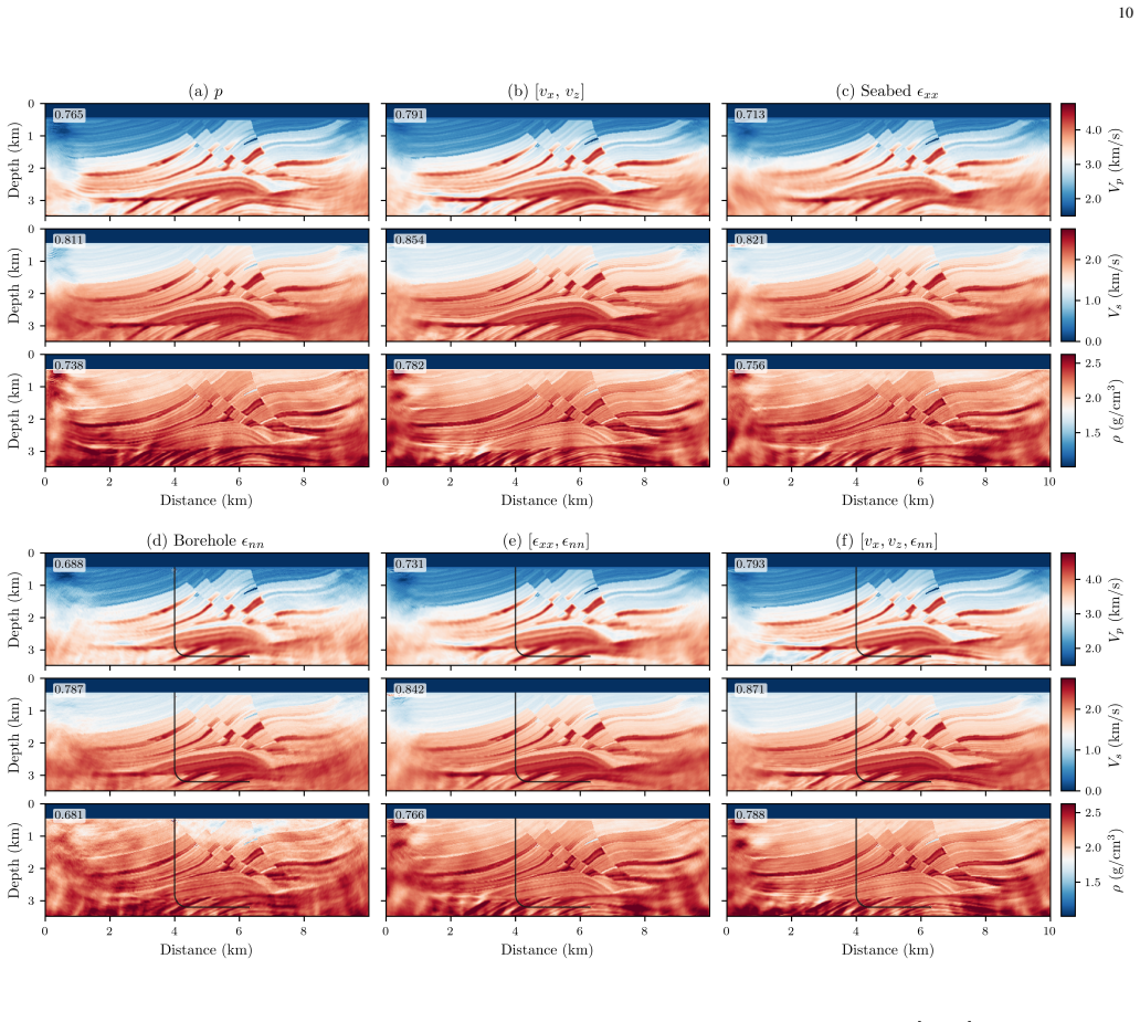
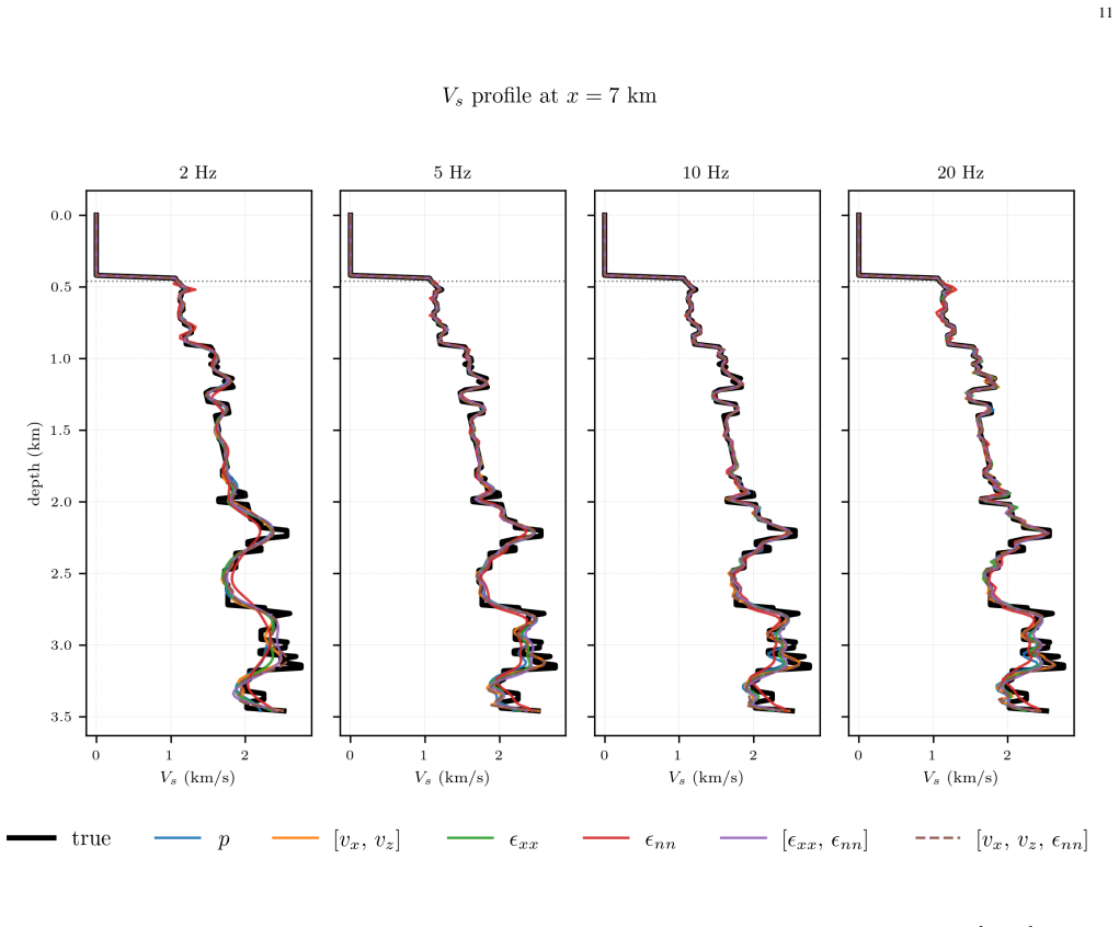
The velocity-stress-strain formulation directly models the physical quantities recorded by both geophones and DAS from a single forward simulation, with residuals from any combination of sensors injected into a single adjoint run whose cost does not grow with the number of active sensor subsets. On the tested models this joint approach recovers elastic parameters more accurately than either sensor type alone, with the combination of two-component geophones and a deviated borehole DAS cable producing the smallest errors and the clearest reduction in cross-talk because the two systems supply distinct physical observables and complementary depth apertures.
What carries the argument
The velocity-stress-strain (VSS) formulation that computes pressure, particle velocity, and gauge-length-averaged DAS strain in one forward simulation and supports additive residual injection in one backward simulation.
If this is right
- Joint use of complementary sensors recovers elastic parameters more accurately than single deployments.
- Computational cost stays constant regardless of which sensor subsets are active.
- Two-component geophones combined with deviated borehole DAS reduce inter-parameter cross-talk most effectively.
- The open-source xFWI package implements the framework for multi-deployment inversions.
Where Pith is reading between the lines
- Acquisition designs could be optimized by deliberately placing geophones and DAS cables to maximize differences in observable type and depth sampling.
- The same single-simulation structure may allow straightforward addition of other sensor types such as pressure hydrophones without changing the adjoint cost scaling.
- Field applications on real data would test whether the synthetic cross-talk reduction holds when sensor coupling and noise characteristics differ from the benchmarks.
Load-bearing premise
The VSS formulation and single backward simulation accurately capture the physics of both sensor types without introducing unmodeled errors.
What would settle it
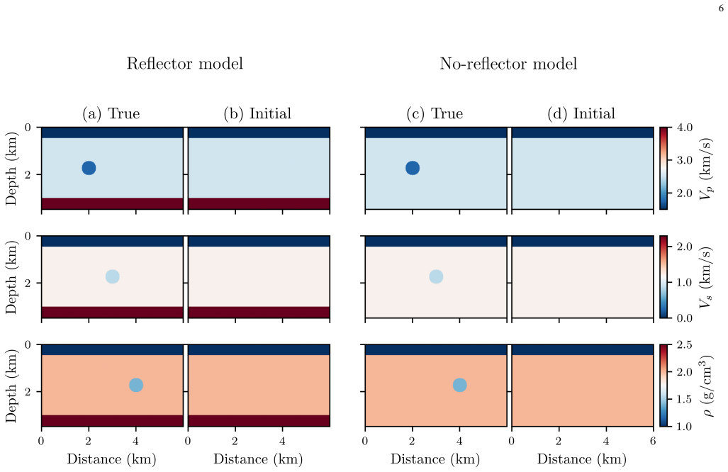
Perform the joint inversion on a known elastic Marmousi model using the stated sensor geometries and measure whether the recovered parameters match the true model within the reported error levels or whether cross-talk between parameters remains visible.
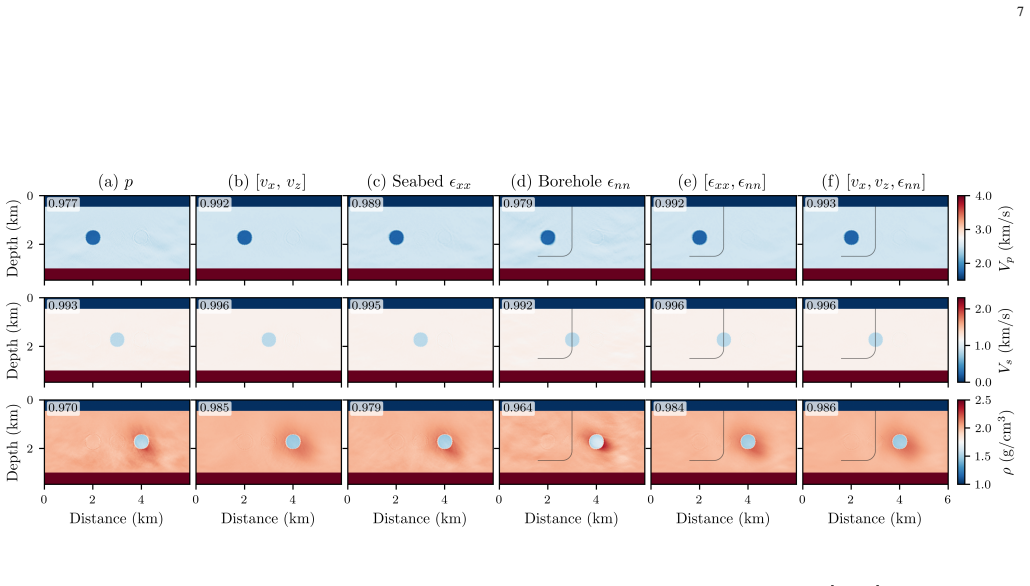
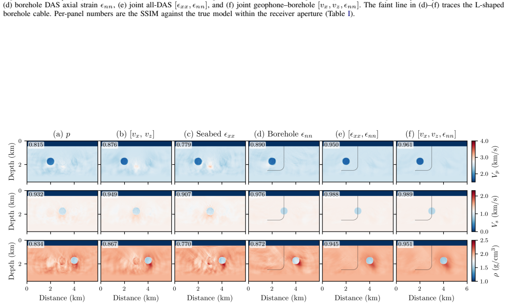
Figures
read the original abstract
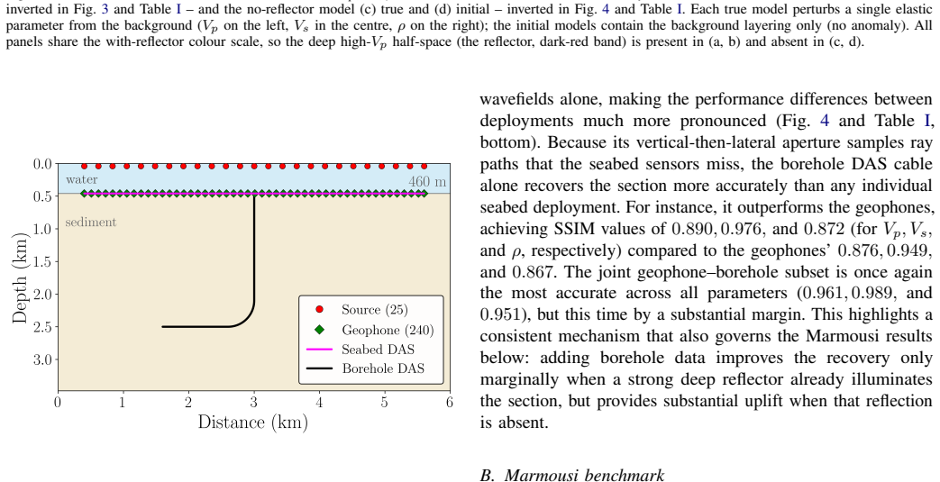
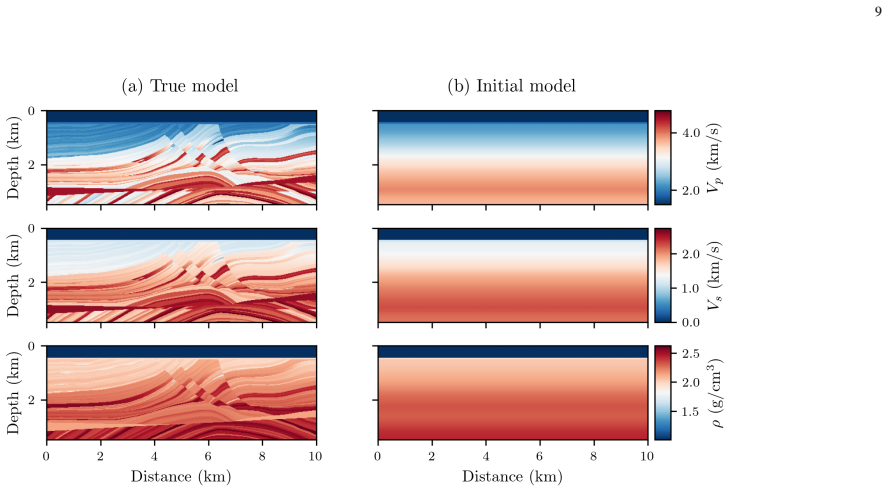
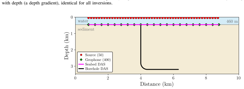
Joint full waveform inversion (FWI) of distributed acoustic sensing (DAS) and ocean-bottom node (OBN) data typically requires converting measured strain to particle velocity, introducing numerical noise and spectral distortion. To eliminate this, we present an elastic multi-parameter FWI framework using a velocity-stress-strain (VSS) formulation that directly models pressure, particle velocity, and gauge-length-averaged DAS strain from a single forward simulation. Data residuals are injected additively into a single backward simulation, making computational cost independent of the active sensor subsets. We benchmark individual and combined datasets on cross-talk and elastic Marmousi models. Our results show that joint inversion recovers elastic parameters more accurately than single deployments when the sensors offer complementary information. Specifically, pairing two-component geophones with a deviated borehole DAS cable yields the most accurate parameter recovery and mitigates inter-parameter cross-talk by providing a distinct physical observable and complementary depth aperture. We release our implementation as xFWI, an open-source, Devito-based Python package for scalable, multi-deployment inversions.
Editorial analysis
A structured set of objections, weighed in public.
Referee Report
Summary. The manuscript presents a velocity-stress-strain (VSS) formulation for joint elastic multi-parameter full waveform inversion (FWI) of multi-component geophone and distributed acoustic sensing (DAS) data. It allows direct modeling of pressure, particle velocity, and DAS strain from a single forward simulation, with additive residual injection in a single backward simulation, making the computational cost independent of the sensor combination. Benchmarks on synthetic cross-talk and elastic Marmousi models show that joint inversion, particularly using two-component geophones paired with a deviated borehole DAS cable, yields superior elastic parameter recovery and reduced inter-parameter cross-talk compared to individual datasets, due to complementary physical observables and depth aperture. The code is released as the open-source xFWI package based on Devito.
Significance. If the synthetic benchmark results generalize, this work could have significant impact on seismic imaging by facilitating efficient joint inversions of heterogeneous sensor data without conversion-induced artifacts. The computational efficiency and open-source implementation are positive aspects that could encourage adoption in the geophysics community for improved subsurface characterization.
minor comments (3)
- [Abstract / Methods] The abstract states that the VSS formulation directly models the observables from a single forward run, but the manuscript should include a brief derivation or reference to the specific strain averaging operator for the DAS gauge length to confirm it introduces no unmodeled spectral effects.
- [Results / Marmousi benchmarks] In the Marmousi benchmark section, the reported accuracy ordering (2C geophone + deviated DAS best) would be strengthened by explicit tabulation of the L2 misfit norms or parameter error percentages for each sensor combination rather than qualitative statements.
- [Computational aspects] The claim that computational cost is independent of active sensor subsets is central; a short complexity table or timing comparison for single vs. joint cases would make this concrete.
Simulated Author's Rebuttal
We thank the referee for their positive summary of our work and for recommending minor revision. Their assessment correctly identifies the key advantages of the VSS formulation for joint multi-deployment elastic FWI.
Circularity Check
No significant circularity
full rationale
The paper's claims rest on synthetic benchmark inversions of the Marmousi model that compare parameter recovery and cross-talk across sensor combinations. The VSS formulation is introduced as an enabling modeling choice that directly produces the required observables (pressure, velocity, strain) from one forward run, with residuals added in the adjoint; the reported superiority of the two-component geophone + deviated DAS pairing follows from the numerical outcomes of those inversions rather than from any redefinition, fitted parameter renamed as prediction, or self-citation chain. No load-bearing step reduces by construction to the paper's own inputs or prior author work.
Axiom & Free-Parameter Ledger
axioms (1)
- standard math Standard elastic wave equations govern pressure, velocity, and strain fields
Reference graph
Works this paper leans on
-
[1]
Ground motion response to an ML 4.3 earthquake using co-located distributed acoustic sensing and seismometer arrays,
H. F. Wang, X. Zeng, D. E. Miller, D. Fratta, K. L. Feigl, C. H. Thurber, and R. J. Mellors, “Ground motion response to an ML 4.3 earthquake using co-located distributed acoustic sensing and seismometer arrays,” Geophysical Journal International, vol. 213, no. 3, pp. 2020–2036, 06
2020
-
[2]
Available: https://doi.org/10.1093/gji/ggy102
[Online]. Available: https://doi.org/10.1093/gji/ggy102
-
[3]
Distributed acoustic sensing for reservoir monitoring with vertical seismic profiling,
A. Mateeva, J. Lopez, H. Potters, J. Mestayer, B. Cox, D. Kiyashchenko, P. Wills, S. Grandi, K. Hornman, B. Kuvshinov, W. Berlang, Z. Yang, and R. Detomo, “Distributed acoustic sensing for reservoir monitoring with vertical seismic profiling,”Geophysical Prospecting, vol. 62, no. 4, pp. 679–692, 2014. [Online]. Available: https://onlinelibrary.wiley.com/d...
-
[4]
Earthquake focal mechanisms with distributed acoustic sensing,
J. Li, W. Zhu, E. Biondi, and Z. Zhan, “Earthquake focal mechanisms with distributed acoustic sensing,”Nature Communications, vol. 14, p. 4181,
-
[5]
Available: https://doi.org/10.1038/s41467-023-39639-3
[Online]. Available: https://doi.org/10.1038/s41467-023-39639-3
-
[6]
Elastic full-waveform inversion: Enhance imaging for legacy and modern acquisition,
F. Liu, C. Macesanu, H. Xing, M. Romanenko, G. Zhan, C. Calder ´on- Mac´ıas, and B. Wang, “Elastic full-waveform inversion: Enhance imaging for legacy and modern acquisition,”The Leading Edge, vol. 44, no. 5, pp. 338–343, 2025. [Online]. Available: https: //doi.org/10.1190/tle44050338.1
-
[7]
An overview of full-waveform inversion in exploration geophysics,
J. Virieux and S. Operto, “An overview of full-waveform inversion in exploration geophysics,” inGeophysics Today: A Survey of the Field as the Journal Celebrates its 75th Anniversary, S. Fomel, Ed. Society of Exploration Geophysicists, 2010, vol. 16, p. 0. [Online]. Available: https://doi.org/10.1190/1.9781560802273
-
[8]
Gauss–Newton and full Newton methods in frequency–space seismic waveform inversion,
R. G. Pratt, C. Shin, and G. J. Hick, “Gauss–Newton and full Newton methods in frequency–space seismic waveform inversion,”Geophysical Journal International, vol. 133, no. 2, pp. 341–362, 05 1998. [Online]. Available: https://doi.org/10.1046/j.1365-246X.1998.00498.x
-
[9]
Seismic imaging of complex onshore structures by 2D elastic frequency-domain full-waveform inversion,
R. Brossier, S. Operto, and J. Virieux, “Seismic imaging of complex onshore structures by 2D elastic frequency-domain full-waveform inversion,”Geophysics, vol. 74, no. 6, pp. WCC105–WCC118, 2009
2009
-
[10]
S. Operto, Y . Gholami, V . Prieux, A. Ribodetti, R. Brossier, L. Metivier, and J. Virieux, “A guided tour of multiparameter full-waveform inversion with multicomponent data: From theory to practice,”The Leading Edge, vol. 32, no. 9, pp. 1040–1054, 09 2013. [Online]. Available: https://doi.org/10.1190/tle32091040.1
-
[11]
Modern case study demonstrations of the industry value of PS-wave data,
A. Tura, R. Yermakov, O. E. Aaker, Ø. Pedersen, A. Damasceno, M. R. Braga, S. L. S. Hoey, L. Ambati, N. N. A. Rahman, S. K. Chandola, A. R. Ghazali, M. F. A. Halim, and B. Olofsson, “Modern case study demonstrations of the industry value of PS-wave data,”First Break, vol. 43, no. 11, pp. 75–84, 2025. [Online]. Available: https: //www.earthdoc.org/content/...
-
[12]
On the influence of model parametrization in elastic full waveform tomography,
D. K ¨ohn, D. De Nil, A. Kurzmann, A. Przebindowska, and T. Bohlen, “On the influence of model parametrization in elastic full waveform tomography,”Geophysical Journal International, vol. 191, no. 1, pp. 325–345, 10 2012. [Online]. Available: https://doi.org/10.1111/j.1365-246X.2012.05633.x
-
[13]
Seismic waveform inversion best practices: regional, global and exploration test cases,
R. Modrak and J. Tromp, “Seismic waveform inversion best practices: regional, global and exploration test cases,”Geophysical Journal International, vol. 206, no. 3, pp. 1864–1889, 09 2016. [Online]. Available: https://doi.org/10.1093/gji/ggw202
-
[14]
Elastic full-waveform inversion and parametrization analysis applied to walk-away vertical seismic profile data for unconventional (heavy oil) reservoir characterization,
W. Pan, K. A. Innanen, and Y . Geng, “Elastic full-waveform inversion and parametrization analysis applied to walk-away vertical seismic profile data for unconventional (heavy oil) reservoir characterization,” Geophysical Journal International, vol. 213, no. 3, pp. 1934–1968, 06
1934
-
[15]
Available: https://doi.org/10.1093/gji/ggy087
[Online]. Available: https://doi.org/10.1093/gji/ggy087
-
[16]
Multiparameter seismic elastic full-waveform inversion with combined geophone and shaped fiber-optic cable data,
M. V . Eaid, S. D. Keating, and K. A. Innanen, “Multiparameter seismic elastic full-waveform inversion with combined geophone and shaped fiber-optic cable data,”Geophysics, vol. 85, no. 6, pp. R537–R552, 11
-
[17]
Available: https://doi.org/10.1190/geo2020-0170.1
[Online]. Available: https://doi.org/10.1190/geo2020-0170.1
-
[18]
Seismic applications of downhole DAS,
A. Lellouch and B. L. Biondi, “Seismic applications of downhole DAS,” Sensors (Basel), vol. 21, no. 9, p. 2897, 04 2021, pMID: 33919095; PMCID: PMC8122346
2021
-
[19]
Distributed acoustic sensing (DAS) to velocity transform and its benefits,
A. Sayed, S. Ali, and R. R. Stewart, “Distributed acoustic sensing (DAS) to velocity transform and its benefits,” inSEG Technical Program Expanded Abstracts 2020. Society of Exploration Geophysicists, 2020, pp. 3788–3792
2020
-
[20]
Direct full waveform inversion of DAS fiber-optic data,
W. Zhou, “Direct full waveform inversion of DAS fiber-optic data,” vol. 2024, no. 1, pp. 1–5, 2024. [Online]. Available: https://www.earthdoc.org/content/papers/10.3997/2214-4609.202410385
-
[21]
P-SV wave propagation in heterogeneous media; velocity- stress finite-difference method,
J. Virieux, “P-SV wave propagation in heterogeneous media; velocity- stress finite-difference method,”Geophysics, vol. 51, no. 4, pp. 889–901, 04 1986. [Online]. Available: https://doi.org/10.1190/1.1442147
-
[22]
D. Komatitsch and R. Martin, “An unsplit convolutional perfectly matched layer improved at grazing incidence for the seismic wave equation,”Geophysics, vol. 72, no. 5, pp. SM155–SM167, 08 2007. [Online]. Available: https://doi.org/10.1190/1.2757586
-
[23]
A. H. Hartog,An Introduction to Distributed Optical Fibre Sensors, 1st ed. Boca Raton: CRC Press, 05 2017. [Online]. Available: https://doi.org/10.1201/9781315119014
-
[24]
Devito (v3.1.0): an embedded domain-specific language for finite differences and geophysical exploration,
M. Louboutin, M. Lange, F. Luporini, N. Kukreja, P. A. Witte, F. J. Herrmann, P. Velesko, and G. J. Gorman, “Devito (v3.1.0): an embedded domain-specific language for finite differences and geophysical exploration,”Geoscientific Model Development, vol. 12, no. 3, pp. 1165–1187, 2019. [Online]. Available: https://gmd.copernicus. org/articles/12/1165/2019/
2019
-
[25]
Architecture and performance of Devito, a system for automated stencil computation,
F. Luporini, M. Lange, M. Louboutin, N. Kukreja, J. H ¨uckelheim, C. Yount, P. Witte, P. H. J. Kelly, F. J. Herrmann, and G. J. Gorman, “Architecture and performance of Devito, a system for automated stencil computation,” 2020. [Online]. Available: https://arxiv.org/abs/1807.03032
-
[26]
O. Holberg, “Computational aspects of the choice of operator and sampling interval for numerical differentiation in large-scale simulation of wave phenomena,”Geophysical Prospecting, vol. 35, no. 6, pp. 629–655, 1987. [Online]. Available: https://onlinelibrary.wiley.com/doi/ abs/10.1111/j.1365-2478.1987.tb00841.x 13
-
[27]
Inversion of seismic reflection data in the acoustic approximation,
A. Tarantola, “Inversion of seismic reflection data in the acoustic approximation,”Geophysics, vol. 49, no. 8, pp. 1259–1266, 08 1984. [Online]. Available: https://doi.org/10.1190/1.1441754
-
[28]
R.-E. Plessix, “A review of the adjoint-state method for computing the gradient of a functional with geophysical applications,”Geophysical Journal International, vol. 167, no. 2, pp. 495–503, 11 2006. [Online]. Available: https://doi.org/10.1111/j.1365-246X.2006.02978.x
-
[29]
A strategy for nonlinear elastic inversion of seismic reflection data,
A. Tarantola, “A strategy for nonlinear elastic inversion of seismic reflection data,”Geophysics, vol. 51, no. 10, pp. 1893–1903, 10 1986. [Online]. Available: https://doi.org/10.1190/1.1442046
-
[30]
Multiscale seismic waveform inversion,
C. Bunks, F. M. Saleck, S. Zaleski, and G. Chavent, “Multiscale seismic waveform inversion,”Geophysics, vol. 60, no. 5, pp. 1457–1473, 10
-
[31]
Available: https://doi.org/10.1190/1.1443880
[Online]. Available: https://doi.org/10.1190/1.1443880
-
[32]
A limited memory algorithm for bound constrained optimization,
R. H. Byrd, P. Lu, J. Nocedal, and C. Zhu, “A limited memory algorithm for bound constrained optimization,”SIAM Journal on Scientific Computing, vol. 16, no. 5, pp. 1190–1208, 1995. [Online]. Available: https://doi.org/10.1137/0916069
-
[33]
Frequency-domain finite-difference amplitude-preserving migration,
R.-E. Plessix and W. A. Mulder, “Frequency-domain finite-difference amplitude-preserving migration,”Geophysical Journal International, vol. 157, no. 3, pp. 975–987, 2004
2004
-
[34]
Dask: Library for dynamic task scheduling,
Dask Development Team, “Dask: Library for dynamic task scheduling,” http://dask.pydata.org, 2016
2016
-
[35]
Slurm: Simple linux utility for resource management,
A. B. Yoo, M. A. Jette, and M. Grondona, “Slurm: Simple linux utility for resource management,” inJob Scheduling Strategies for Parallel Processing, D. Feitelson, L. Rudolph, and U. Schwiegelshohn, Eds. Berlin, Heidelberg: Springer Berlin Heidelberg, 2003, pp. 44–60
2003
-
[36]
Image quality assessment: from error visibility to structural similarity,
Z. Wang, A. C. Bovik, H. R. Sheikh, and E. P. Simoncelli, “Image quality assessment: from error visibility to structural similarity,”IEEE Transactions on Image Processing, vol. 13, no. 4, pp. 600–612, 04 2004, pMID: 15376593
2004
-
[37]
Marmousi2: An elastic upgrade for Marmousi,
G. S. Martin, R. Wiley, and K. J. Marfurt, “Marmousi2: An elastic upgrade for Marmousi,”The Leading Edge, vol. 25, no. 2, pp. 156–166, 02 2006. [Online]. Available: https://doi.org/10.1190/1.2172306
discussion (0)
Sign in with ORCID, Apple, or X to comment. Anyone can read and Pith papers without signing in.