Iterated Tikhonov regularization of large linear problems
Pith reviewed 2026-06-30 04:44 UTC · model grok-4.3
The pith
Partial Golub-Kahan bidiagonalization determines the regularization parameter for iterated Tikhonov regularization via Gauss quadrature without computing multiple solutions.
A machine-rendered reading of the paper's core claim, the machinery that carries it, and where it could break.
Core claim
Iterated Tikhonov regularization based on partial Golub-Kahan bidiagonalization can determine the regularization parameter without computing several approximate solutions by using the connection between Golub-Kahan bidiagonalization and Gauss quadrature. This approach reduces the computational effort required to compute a desired solution that satisfies the discrepancy principle.
What carries the argument
The connection between partial Golub-Kahan bidiagonalization and Gauss quadrature, used to estimate the value of the regularization parameter that makes the residual norm match the known data error norm.
If this is right
- A single run of the bidiagonalization process yields both an approximate solution and the needed parameter value.
- The method inherits the higher accuracy typical of iterated Tikhonov regularization while lowering the cost of parameter selection.
- The approach scales to large problems because only a modest number of bidiagonalization steps are required.
- No explicit formation of the full normal equations or repeated factorizations is needed.
Where Pith is reading between the lines
- The same quadrature link might be adapted to other iterative regularization families that rely on bidiagonalization.
- In applications where the error norm estimate is updated during computation, the method could be re-run with modest extra cost.
- The technique could be combined with early stopping criteria to further limit the number of matrix-vector products.
Load-bearing premise
The Gauss quadrature connection supplied by the bidiagonalization process accurately identifies a regularization parameter that satisfies the discrepancy principle.
What would settle it
A numerical test on a standard ill-posed problem where the quadrature estimate produces a residual norm that deviates from the known error norm by more than the discrepancy tolerance.
Figures
read the original abstract
Many solution methods for linear discrete ill-posed problems with error-contaminated data (right-hand side) apply Tikhonov regularization to compute a meaningful approximate solution. This solution depends on a regularization parameter. It is well known that iterated Tikhonov regularization often determines an approximate solution of higher quality than (standard) Tikhonov regularization. We consider the situation when an estimate of the norm of the error in the data is known and would like to apply iterative Tikhonov regularization to determine an approximate solution that satisfies the discrepancy principle. This requires a suitable choice of a regularization parameter. The standard approach to determine this parameter is to compute solutions for several values of the regularization parameter and choose a computed approximate solution that satisfies the discrepancy principle. This paper discusses iterated Tikhonov regularization based on partial Golub-Kahan bidiagonalization and describes how the regularization parameter can be determined without computing several approximate solutions by using the connection between Golub-Kahan bidiagonalization and Gauss quadrature. This approach reduces the computational effort required to compute a desired solution.
Editorial analysis
A structured set of objections, weighed in public.
Referee Report
Summary. The paper proposes iterated Tikhonov regularization for large linear discrete ill-posed problems with known noise level. It employs partial Golub-Kahan bidiagonalization and the link to Gauss quadrature to select the regularization parameter satisfying the discrepancy principle, avoiding explicit computation of multiple approximate solutions for different parameter values and thereby reducing computational effort compared to the standard approach.
Significance. If the central derivation holds, the work extends the established Golub-Kahan/Gauss-quadrature connection (previously used for standard Tikhonov and LSQR) to the iterated setting. This yields a parameter-free way to evaluate the discrepancy functional from bidiagonalization quantities alone, which is a practical efficiency gain for large-scale inverse problems where repeated solves are prohibitive.
minor comments (2)
- [Abstract / Method description] The abstract and method description would benefit from an explicit statement of the iterated filter factors in terms of the bidiagonalization quantities (e.g., a displayed equation analogous to the standard Tikhonov case) to make the quadrature reuse immediately verifiable.
- A short numerical example or complexity count comparing the new approach to the conventional multi-λ search would strengthen the claim of reduced effort; its absence leaves the efficiency statement qualitative.
Simulated Author's Rebuttal
We thank the referee for the positive summary and significance assessment of our work on extending the Golub-Kahan/Gauss-quadrature approach to iterated Tikhonov regularization. The recommendation of minor revision is noted.
Circularity Check
No significant circularity detected
full rationale
The paper extends the established Golub-Kahan bidiagonalization–Gauss quadrature connection (previously used for standard Tikhonov) to iterated Tikhonov so that the discrepancy principle can be evaluated from bidiagonalization quantities alone. The abstract and method description indicate that iterated filter factors are expressed via the same tridiagonal structure, allowing quadrature reuse. No self-definitional equations, fitted inputs renamed as predictions, or load-bearing self-citation chains appear; the central claim rests on an independent, externally verifiable mathematical link applied to a new regularization variant. The derivation is therefore self-contained against external benchmarks.
Axiom & Free-Parameter Ledger
Reference graph
Works this paper leans on
-
[1]
The use of auto-correlation for pseudo-r ank determination in noisy ill-conditioned least-squares problems
Baart, M.L., 1982. The use of auto-correlation for pseudo-r ank determination in noisy ill-conditioned least-squares problems. IMA J. Numer. Anal. 2, 241–247
1982
-
[2]
T he iterated golub-kahan-tikhonov method
Bianchi, D., Donatelli, M., Furchì, D., Reichel, L., 2026. T he iterated golub-kahan-tikhonov method. BIT Numer. Math. 66, 18. Björck, A., 1988. A bidiagonalization algorithm for solvin g large and sparse ill-posed systems of linear equations. BI T Numer. Math. 18, 659–670
2026
-
[3]
Regularizing preconditioners by non-st ationary iterated tikhonov with general penalty term
Buccini, A., 2017. Regularizing preconditioners by non-st ationary iterated tikhonov with general penalty term. Appl . Numer. Math. 116, 64–81
2017
-
[4]
Iterated tik honov regularization with a general penalty term
Buccini, A., Donatelli, M., Reichel, L., 2017. Iterated tik honov regularization with a general penalty term. Numer. Li near Algebra Appl. 24, e2089
2017
-
[5]
An arnoldi-based preconditioner for iterated tikhonov regularization
Buccini, A., Onisk, L., Reichel, L., 2023. An arnoldi-based preconditioner for iterated tikhonov regularization. Num er. Algorithms 92, 223–245
2023
-
[6]
Generalized sing ular value decomposition with iterated tikhonov regulariz ation
Buccini, A., Pasha, M., Reichel, L., 2020. Generalized sing ular value decomposition with iterated tikhonov regulariz ation. J. Comput. Appl. Math. 373, 112276
2020
-
[7]
Estimation of the l-curve via lanczos bidiagonalization
Calvetti, D., Golub, G.H., Reichel, L., 1999. Estimation of the l-curve via lanczos bidiagonalization. BIT Numer. Math . 39, 603–619
1999
-
[8]
Tikhonov regularization o f large linear problems
Calvetti, D., Reichel, L., 2003. Tikhonov regularization o f large linear problems. BIT Numer. Math. 43, 263–283
2003
-
[9]
Computational methods for lar ge-scale inverse problems: A survey on hybrid projection me thods
Chung, J., Gazzola, S., 2024. Computational methods for lar ge-scale inverse problems: A survey on hybrid projection me thods. SIAM Rev. 66, 205–284
2024
-
[10]
Square smoothing regular ization matrices with accurate boundary conditions
Donatelli, M., Reichel, L., 2014. Square smoothing regular ization matrices with accurate boundary conditions. J. Com put. Appl. Math. 272, 334–349
2014
-
[11]
Regul arization matrices for discrete ill-posed problems in several space-dimensions
Dykes, L., Huang, G., Noschese, S., Reichel, L., 2018. Regul arization matrices for discrete ill-posed problems in several space-dimensions. Numer. Linear Algebra Appl. 25, e2163. Eldén, L., 1982. A weighted pseudoinverse, generalized sin gular values, and constraint least squares problems. BIT Nu mer. Math. 22, 487–502
2018
-
[12]
Regularization o f Inverse Problems
Engl, H.W., Hanke, M., Neubauer, A., 1996. Regularization o f Inverse Problems. Dordrecht
1996
-
[13]
Ir tools: a matl ab package of iterative regularization methods and large-s cale test problems
Gazzola, S., Hansen, P.C., Nagy, J.G., 2019. Ir tools: a matl ab package of iterative regularization methods and large-s cale test problems. Numer. Agorithms 81, 773–811
2019
-
[14]
Matrices, Moments and Quadr ature with Applications
Golub, G.H., Meurant, G., 2010. Matrices, Moments and Quadr ature with Applications. Princeton University Press, Prin ceton
2010
-
[15]
Regularization tools: A matlab package for analysis and solution of discrete ill-posed problems
Hansen, P.C., 1994. Regularization tools: A matlab package for analysis and solution of discrete ill-posed problems. N umer. Agorithms 6, 1–35
1994
-
[16]
Rank-Deficient and Discrete Ill-Posed P roblems
Hansen, P.C., 1998. Rank-Deficient and Discrete Ill-Posed P roblems. SIAM, Philadelphia
1998
-
[17]
Application of denoising me thods to regularization of ill-posed problems
Hearn, T.A., Reichel, L., 2014. Application of denoising me thods to regularization of ill-posed problems. Numer. Agor ithms 66, 761–777
2014
-
[18]
Image denoising via residua l kurtosis minimization
Hearn, T.A., Reichel, L., 2015. Image denoising via residua l kurtosis minimization. Numer. Math. Theor. Meth. Appl. 8, 403–422
2015
-
[19]
Convergence analysis of minimizatio n-based noise level-free parameter choice rules for linear ill-posed problems
Kindermann, S., 2011. Convergence analysis of minimizatio n-based noise level-free parameter choice rules for linear ill-posed problems. Electron. Trans. Numer. Anal. 38, 233–257
2011
-
[20]
A simplified l-curve method a s error estimator
Kindermann, S., Raik, K., 2020. A simplified l-curve method a s error estimator. Electron. Trans. Numer. Anal. 53, 217–23 8. López Lagomasino, G., Reichel, L., Wunderlich, L., 2008. Ma trices, moments, and rational quadrature. Linear Algebra A ppl. 429, 2540–2554
2020
-
[21]
Orthogonal pro jection regularization operators
Morigi, S., Reichel, L., Sgallari, F., 2007. Orthogonal pro jection regularization operators. Numer. Agorithms 44, 99 –114
2007
-
[22]
An a posteriori parameter choice for tik honov regularization in the presence of modeling errors
Neubauer, A., 1998. An a posteriori parameter choice for tik honov regularization in the presence of modeling errors. Ap pl. Numer. Math. 4, 507–519
1998
-
[23]
Lsqr: An algorithm for sp arse linear equations and sparse least squares
Paige, C.C., Saunders, M.A., 1982. Lsqr: An algorithm for sp arse linear equations and sparse least squares. ACM Trans. M ath. Software 8, 43–71
1982
-
[24]
Old and new parameter choi ce rules for discrete ill-posed problems
Reichel, L., Rodriguez, G., 2013. Old and new parameter choi ce rules for discrete ill-posed problems. Numer. Agorithms 63, 65–87
2013
-
[25]
Greedy tikhonovregularization for large linear ill-posed problems
Reichel, L., Sadok, H., Shyshkov, A., 2007. Greedy tikhonovregularization for large linear ill-posed problems. Int. J. Comput. Math. 84, 1151–1166
2007
-
[26]
A new zero-finder for tikhon ov regularization
Reichel, L., Shyshkov, A., 2008. A new zero-finder for tikhon ov regularization. BIT Numer. Math. 48, 627–643
2008
-
[27]
Improvements of the resolution of an instrument by numerical solution of an integral equation
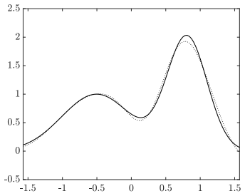
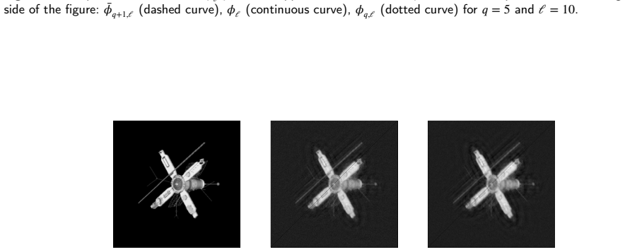
Shaw, C.B.J., 1972. Improvements of the resolution of an instrument by numerical solution of an integral equation. J. Ma th. Anal. Appl. 37, 83–112. D. Furchì and L. Reichel: Preprint submitted to Elsevier Page 13 of 13 Figure 1: Example 5.1: Solution /uni0302.s1/u1D499of the error-free linear system ( 3) (continuous curve) and computed approximate soluti...
1972
discussion (0)
Sign in with ORCID, Apple, or X to comment. Anyone can read and Pith papers without signing in.