Classification and prediction of wave chaotic systems with machine learning techniques

Bisrat Addissie; Bo Xiao; Edward Ott; Ron Hong; Shukai Ma; Steven Anlage; Thomas Antonsen; Zachary Drikas

REVIEW 2 major objections 5 minor 50 references

Classification and prediction of wave chaotic systems with machine learning techniques

T0 review · 2 major / 5 minor · reviewed 2026-08-14 · deepseek-v4-flash

Challenge this review Re-run · record.json Download PDF Read on arXiv ↗ Review JSON

Pith's one-line read Machine learning can classify the number of connected wave chaotic cavities from raw reflection spectra and can forecast future transmission with a recurrent network.

desk verdict The classification half is a solid, citable result; the RNN forecasting half is undermined by the mode-stirrer periodicity because the test realizations repeat training phases, so the prediction claim should be treated as unsubstantiated until reworked. read the letter →

arxiv 1908.04716 v1 pith:NDA3C526 submitted 2019-08-13 cond-mat.dis-nn nlin.CD

Shukai Ma , Bo Xiao , Ron Hong , Bisrat Addissie , Zachary Drikas , Thomas Antonsen , Edward Ott , Steven Anlage This is my paper · ORCID

classification cond-mat.dis-nnnlin.CD

keywords wavechaosmachinelearningneuralnetworkscatteringmatrixmicrowavecavitiesrecurrentrandomcouplingmodelmodestirrer

verification ladder T0 review T1 audit T2 compute T3 formal

The pith

A machine-rendered reading of the paper's core claim, the machinery that carries it, and where it could break.

The reading

The paper tests whether model-free machine learning can see structure in wave chaotic scattering that standard statistics miss. Using measured microwave reflection spectra from cascades of one, two, or three connected lossy cavities, a supervised neural network is trained to label the number of cavities; with all 16,001 frequency points as input, held-out test accuracy reaches 100 percent. The same network degrades gracefully under added noise and refuses to extrapolate to a cavity-count class it never saw during training. The paper also trains a recurrent neural network on the first 900 realizations of a rotating mode-stirrer sequence and finds that it predicts the measured transmission magnitude for roughly the next 40 realizations from later reflection data alone. Together the results argue that raw scattering data carry hidden system-level information that a trained algorithm can exploit for both classification and short-horizon prediction.

What carries the argument

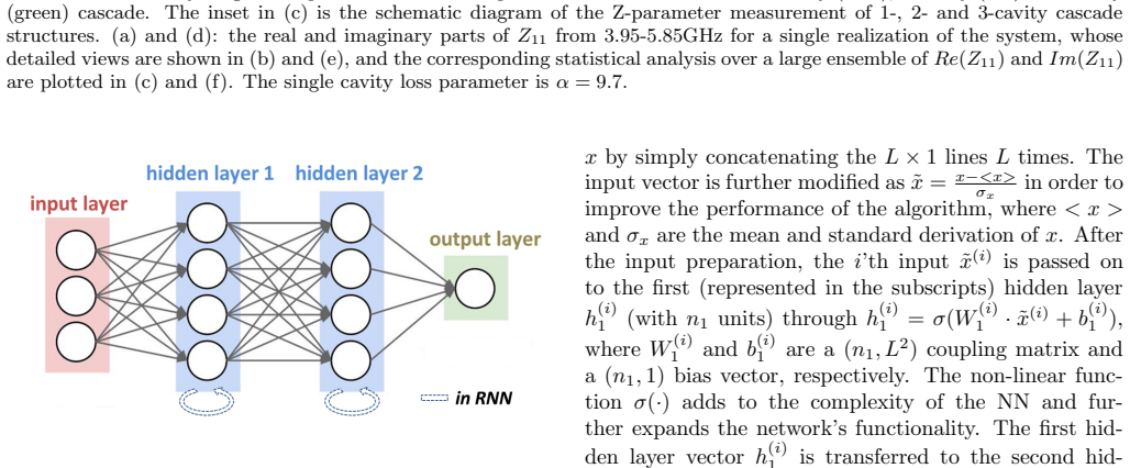
The load-bearing object is the trained neural network itself. For classification, a feedforward network with four hidden layers (25, 26, 33, and 18 units) receives a normalized raw spectrum $\tilde{x}=(x-\langle x\rangle)/\sigma_x$ as input and outputs a one-hot three-class vector; training minimizes a cost function by back-propagation, and the frequency-resolved inputs carry the information that statistical summaries discard. For prediction, a layer-recurrent network adds feedback loops $h^{(i)}=\sigma(W_{x\to h}x^{(i)}+W_{h\to h}h^{(i-1)}+b)$ to one hidden layer of 38 units, so the hidden state carries memory of the previous stirrer realizations; this memory is what lets the network translate a later reflection measurement into a transmission forecast. Input standardization and minimization of the prediction error during training complete the mechanism.

What would settle it

Measure a fresh set of realizations beyond the original 1000, starting at a stirrer angle not contained in the first 900, feed the same trained RNN the reflection data, and compare predicted to measured transmission; if prediction errors jump to chance level on those never-seen phases while remaining low on phase repeats, the forecasting claim would be shown to rest on memorized periodicity rather than extrapolation. For the classification claim, a direct check is to train on data with randomly permuted frequency labels: if accuracy persists under scrambling, the network is using something other than spectral structure.

Watch

Extended reading notes

Core claim

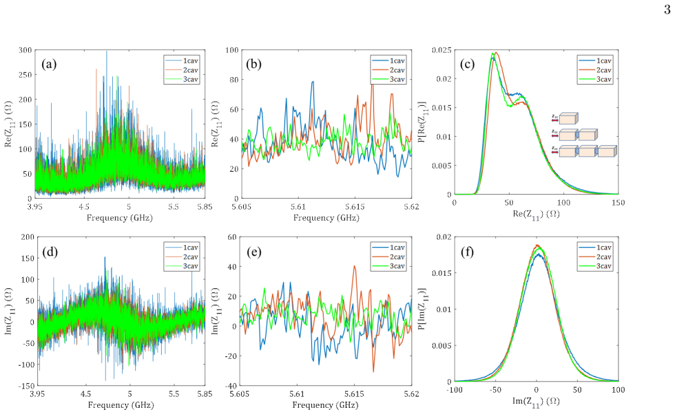
The central claim is that supervised neural networks can uncover hidden order in raw scattering data of wave chaotic systems, where visual inspection and standard statistical analyses fail. For the cascade experiment, the diagonal impedance Re(Z11) of 1-, 2-, and 3-cavity systems has nearly identical probability distributions and mean values (the mean varies by 0.7 percent), yet a four-hidden-layer network trained on 80 percent of 600 realizations classifies the held-out 20 percent perfectly when the full frequency sweep is used. The paper additionally claims that a recurrent neural network with 38 hidden units, trained on the ordered sequence of |S11| at 50 frequencies and |S21| at 5 frequencies, can act as an observer: fed measured |S11| from later realizations, it outputs |S21| that tracks the measured values for the first 40 or so of the 100 test realizations. The authors frame the classification as detecting details not easily summarized by statistical moments, and the prediction as an extension of recent machine-learning forecasting of chaotic systems.

Load-bearing premise

The forecasting result rests on the assumption that the test realizations (901 through 1000) are genuinely unseen future states, even though a full mode-stirrer rotation takes about 120 steps, so the training set of 900 realizations already covers seven and a half rotations and the test interval revisits stirrer phases already encountered; the paper acknowledges some correlations but does not quantify or exclude periodic repeat.

Editorial extensions

If this is right

A single measured reflection spectrum, not an ensemble average, suffices to label the number of connected cavities in a weakly coupled lossy cascade.
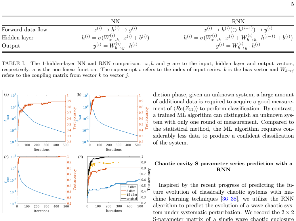
Classification quality improves with spectral resolution: accuracy climbs from 95 percent with 2,000 input points to 98.3 percent with 5,000 points and to 100 percent with all 16,001 points.
The trained classifier is robust to moderate noise: at +15 dB SNR accuracy stays near 0.9, falling to 0.66 at -5 dB.
The classifier generalizes only within its training ensemble; unseen 2-cavity data are assigned equally to all classes, showing the network does not invent categories.
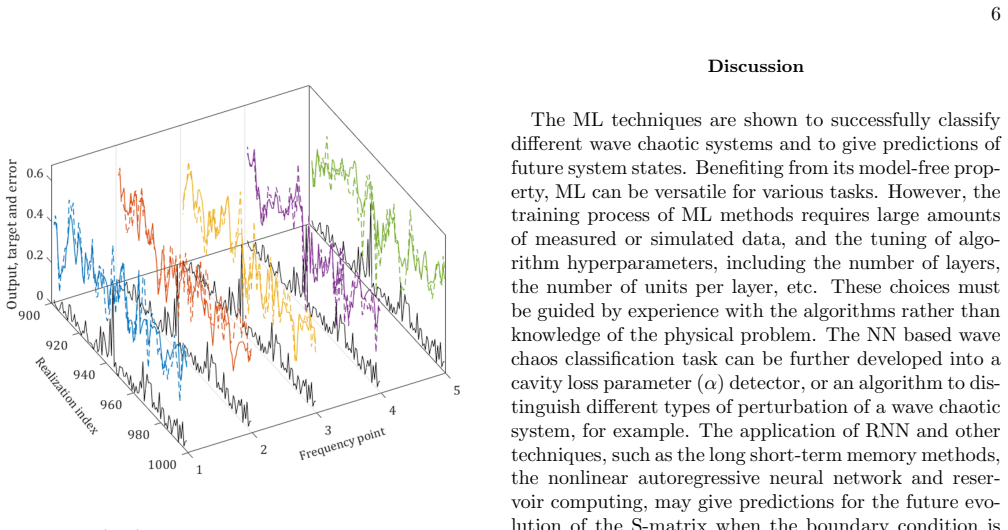
For a systematically rotated mode stirrer, the recurrent network forecasts transmission from reflection for roughly the first 40 future realizations before the error grows large.

Reading between the lines

Editorial extensions of the paper, not claims the author makes directly.

Because a full stirrer rotation takes about 120 steps and training spans 900 steps, the test interval 901 through 1000 revisits stirrer phases that appeared in training, so the forecasting result may reflect interpolation or periodic-memory effects rather than extrapolation; a test on a fresh rotation cycle beyond step 1000 would separate these.
The classification network's access to 16,001 frequency points suggests it uses frequency-resolved interference details rather than single-frequency statistics; one testable extension is to train on synthetic cascades generated by the random coupling model to see which features drive the decision.
The same architecture could be retrained to output other hidden parameters, such as the random-coupling-model loss parameter or the type of boundary perturbation, providing a general scattering-fingerprint tool for enclosures.
The reflection-in, transmission-out observer relation could be applied to detect coherent perfect absorption conditions in real time, as the authors note; a practical extension would be to test prediction horizons against stirrer rotation speed and loss.

Share X Bluesky LinkedIn Reddit HN

Signed reviews

No signed human review yet.

Editorial analysis

A structured set of objections, weighed in public.

Desk editor's note, referee report, and a circularity audit.

Desk Editor's Note

read the letter

Quick take: the paper's real contribution is the classification half. A feedforward net trained on raw Re(Z11) spectra from one-, two-, and three-cavity chains reaches 100% held-out accuracy with full 16001-point inputs, 98.3% with 5000 points, and the authors show the standard statistical summaries (PDFs, mean values) cannot separate these cases. They also include a sensible negative control (an unseen class maps to roughly equal probabilities) and a noise robustness curve. That is an honest, useful proof of concept, and the claim that the net finds structure not captured by hand-built statistics is credible.

The forecasting half does not hold up as stated. The single-cavity sequence comes from a rotating mode stirrer with a ~120-step full rotation. Training on realizations 1-900 and testing on 901-1000 means every test realization repeats a stirrer phase already seen in training (901+i has the phase of 61+i). The authors mention 'some correlations' and then report good agreement for the first ~40 test realizations. That is exactly what periodic recall would look like. There is no baseline, no quantitative error metric, and no evidence the RNN does better than a lag-120 persistence or linear predictor. This is not a minor caveat; it is the difference between extrapolation and interpolation, and the title and abstract claim prediction.

The classification experiments use only 200 realizations per class and a fixed set of hyperparameters; that is fine for a proof of concept, but the paper would be stronger with cross-validation and a statement about how the train/test split was made. Lack of code/data availability is a minor annoyance, not a flaw. The references are appropriate and not self-citation heavy.

Who this is for: people working on ML for scattering, EMC, or wave chaos. The classification result deserves serious peer review and publication. The forecasting claim needs to be reworked before it is publishable. A serious referee should send it back with a request for a baseline and a non-periodic or phase-decorrelated test. I would accept it for review because the classification half is solid and the forecasting error is instructive.

Referee Report

2 major / 5 minor

Summary. The paper reports two machine learning experiments on wave chaotic microwave cavities. In the first, a feedforward neural network is trained to classify the number of connected cavities (1, 2, or 3) from raw measured reflection spectra, achieving 100% test accuracy when all 16001 frequency points are used; the authors also examine robustness to Gaussian noise and to an unseen cavity class. In the second, a recurrent neural network is trained on the first 900 of 1000 realizations of a single cavity's S-parameters under sequential mode-stirrer rotation and is claimed to predict future |S21| values from measured |S11| for roughly the next 40 realizations. The classification experiment is supported by held-out testing, but the forecasting experiment is compromised by the mode stirrer's stated ~120-step periodicity, which aligns the phases of test realizations 901-940 with training realizations 61-100.

Significance. The classification result is a genuine and well-executed demonstration that supervised machine learning can extract hidden structural information from raw scattering data in a regime where conventional statistical descriptors are virtually indistinguishable; this is of interest for electromagnetic compatibility and wave chaotic scattering applications. The forecasting claim, if properly established, would be a notable step toward predicting the response of perturbed complex systems, but as presented it is not supported because of the phase-overlap problem and the absence of quantitative baselines. The paper's overall contribution therefore reduces to the classification result, which is sound but modest; the forecasting portion needs substantial revision before it can be credited.

major comments (2)

[Section IV, 'Chaotic cavity S-parameter series prediction with a RNN'] The RNN forecasting experiment is compromised by the periodicity of the mode stirrer. The text states that a full rotation of the stirrer takes about 120 steps and that the first 900 realizations are used for training. Since 840 = 7 × 120, the test realizations 901 through 940 have exactly the same stirrer phases as training realizations 61 through 100. The apparent agreement in Fig. 5 for the first ~40 realizations is therefore consistent with the network recalling a periodic pattern rather than extrapolating to genuinely unseen dynamics. The authors acknowledge "some correlations between the measurements" but neither quantify them nor compare against a trivial periodic-lag baseline (e.g., the measured |S21| from the corresponding phase one period earlier). Please add such a baseline, and/or redesign the split so that test phases are not present in training (for instance, train on a subset of phases and test on a phase interval never encountered during training), and report quantitative errors. Without this, the forecasting claim in the abstract and conclusion is not established.
[Section IV, 'Chaotic cavity S-parameter series prediction with a RNN'] Even setting aside the phase-overlap issue, the evaluation of the RNN is informal. The paper reports "good agreement" for the first ~40 realizations in Fig. 5, but gives no scalar error metric, no comparison with a null model, and no explicit prediction horizon in units of stirrer steps. A quantitative assessment (for example, normalized mean squared error versus the measured |S21|, and against baselines such as the last training realization or the periodic-lag prediction) is necessary to substantiate the claim of successful prediction.

minor comments (5)

[Section IV, 'Chaotic cavity S-parameter series prediction with a RNN'] The input description "50 frequency points with 175MHz spacing from 75-110 GHz" is internally inconsistent: 50 points at 175 MHz spacing cover only 8.575 GHz, not the stated 35 GHz span. Similarly, "5 frequency points with 2.5GHz spacing" would cover 10 GHz, not the entire band. Please clarify the actual frequency sampling used.
[Section III] The nonlinear activation function σ(·) is never specified, and important training hyperparameters (learning rate, number of epochs, optimizer settings) are not reported. Including these details would improve reproducibility.
[Section IV, 'Cascaded multi-cavity system classification'] In the noise robustness test, the text says the final test accuracy changed from 0.9 to 0.66, but the listed SNR values are +15, 5, and -5 dB; please make the correspondence between accuracy and SNR explicit.
[Section II] The bilinear transformation formula appears garbled: "S = Z0^0.5 (Z + Z0)^-1 (Z - Z0) Z0^0.5" is missing an operator and the ordering of terms is unclear. Please correct and write the expression in a standard form.
[Section IV, 'Cascaded multi-cavity system classification'] The statement that "the algorithm utilizes details that are not easily summarized when making a high resolution distinction" is plausible, but the evidence would be strengthened by reporting the actual values of the mean Re(Z11) differences and the classification accuracy after normalization by the average, which is already performed but not presented as a table or explicit number.

Circularity Check

1 steps flagged · score 6.0 of 10

RNN 'future state' forecast is periodic with training data: every test realization 901-1000 shares a mode-stirrer phase seen in realizations 1-900, so the forecasting claim is partly circular; the classification result remains independently supported.

fitted input called prediction [Section IV, 'Chaotic cavity S-parameter series prediction with a RNN', p. 5-6]
"The mode stirrer is rotated to 1000 unique angles with uniform step angle size. A full rotation of the mode stirrer takes ∼ 120 steps. There exists some correlations between the measurements. ... The first 900 realization of the measured data are used as the training set, and the testing begins with the 901’st realization."

The paper's own numbers make the test set equivalent to training states by construction: 901 = 7×120 + 61 and 1000 = 8×120 + 40, so every stirrer phase in the 901-1000 test block (phases 61-120 and 1-40 modulo 120) already occurred among the 900 training realizations. A mode-stirrer configuration repeats after about 120 steps, so the S-parameters at those phases are near repeats of training measurements. The RNN can therefore achieve the reported agreement by recalling periodic structure embedded in the training data rather than by forecasting genuinely unseen wave-chaotic configurations.

full rationale

The classification half of the paper is self-contained and not circular: 80% of 600 measured realizations are used to train a feedforward network and 20% are held out, with test accuracies of 95-100% depending on input size; the held-out realizations are not used in training, so the 100% full-spectrum test accuracy is a genuine out-of-sample result. The circularity is localized to the RNN forecasting experiment. Because the single-cavity mode stirrer has a stated period of about 120 steps, the 100 test realizations (901-1000) all have stirrer phases that appeared in the 900 training realizations (901-840=61 and 840=7×120; similarly through 1000). Thus the 'future' is composed of near-repeated configurations, not unseen states. The authors explicitly note correlations but neither quantify the overlap nor compare against the trivial baseline of copying the previous period. Since forecasting is advertised in the title and abstract as a central contribution, this is a partial circularity: one of the two main claims reduces to interpolation or memorization of periodic training data. The several self-citations to RCM and reservoir-computing works are background and motivational, not load-bearing derivations, and do not contribute additional circularity.

Assumptions & free parameters 5 free parameters · 4 assumptions · 0 invented entities

The paper introduces no new physical entities or free physics parameters; the fitted quantities are neural-network hyperparameters and input choices. The central scientific burden is carried by experimental data and standard supervised learning. The most consequential 'axiom' is the periodic-stirrer assumption, which creates the data leakage that threatens the forecasting claim.

free parameters (5)

NN hidden layer sizes = [25, 26, 33, 18]
Chosen by hand for the classification network; the paper states the choice 'can be varied', so it is not derived from data or theory.
RNN hidden units = 38
Chosen for the single-hidden-layer recurrent network; no selection procedure is given.
Classification input size = 2000, 5000, 16001 frequency points
The authors test three input vector lengths and report higher accuracy for longer inputs; the final 100% result uses the full 16001 points.
Train/test split = 80/20 for classification; 900/100 for RNN
Split is chosen by the authors; the RNN test portion overlaps in stirrer phase with training because 900 is a multiple of the ~120-step rotation period.
Output frequency subset for RNN = 5 points at 2.5 GHz spacing
The prediction task is defined only for these five transmission frequencies; generalization to other frequencies is not shown.

assumptions (4)

domain assumption The wave chaotic enclosures are well described by random matrix theory and the Random Coupling Model (ergodic, loss parameter alpha=9.7).
The paper relies on RCM statistics to argue that multi-cavity Z11 distributions are nearly indistinguishable, motivating the ML approach (Sections I and II).
domain assumption Mode-stirrer rotations generate statistically independent realizations for the classification ensemble.
The classification experiment assumes 200 stirrer angles give distinct, low-correlation configurations; the paper states stirrers are rotated to ensure low correlation but does not quantify it.
domain assumption The S-parameter measurements are accurate and reproducible at the level needed to train and test the networks.
The VNA data are used without uncertainty quantification; calibration errors would directly affect the reported accuracies (Section II).
domain assumption A full stirrer rotation is 120 steps and the sequence is systematic, so realizations separated by 120 steps are physically related.
The RNN prediction hinges on this periodicity; the paper acknowledges 'some correlations' but does not model them (Section IV).

how reviews work

0 comments

Cite this review

Pith. "Pith review of Classification and prediction of wave chaotic systems with machine learning techniques." pith.science (2026). https://pith.science/paper/NDA3C526

@misc{pith2026190804716,
  author       = {Pith},
  title        = {Pith review of: Classification and prediction of wave chaotic systems with machine learning techniques},
  year         = {2026},
  howpublished = {\url{https://pith.science/paper/NDA3C526}},
  note         = {Machine review of arXiv:1908.04716}
}

read the original abstract

The wave properties of complex scattering systems that are large compared to the wavelength, and show chaos in the classical limit, are extremely sensitive to system details. A solution to the wave equation for a specific configuration can change substantially under small perturbations. Due to this extreme sensitivity, it is difficult to discern basic information about a complex system simply from scattering data as a function of energy or frequency, at least by eye. In this work, we employ supervised machine learning algorithms to reveal and classify hidden information about the complex scattering system presented in the data. As an example we are able to distinguish the total number of connected cavities in a linear chain of weakly coupled lossy enclosures from measured reflection data. A predictive machine learning algorithm for the future states of a perturbed complex scattering system is also trained with a recurrent neural network. Given a finite training data series, the reflection/transmission properties can be forecast by the proposed algorithm.

Figures

Figures reproduced from arXiv: 1908.04716 by the authors.

**Figure 2.** FIG. 2. Multi-cavity diagonal impedances [PITH_FULL_IMAGE:figures/full_fig_p003_2.png] view at source ↗

**Figure 3.** FIG. 3. Generalized (recurrent) neural network architecture [PITH_FULL_IMAGE:figures/full_fig_p003_3.png] view at source ↗

Figures from the paper (2 more)

**Figure 4.** Figure 4: FIG. 4. The NN classification algorithm performance for [PITH_FULL_IMAGE:figures/full_fig_p005_4.png]

**Figure 5.** Figure 5: FIG. 5. The [PITH_FULL_IMAGE:figures/full_fig_p006_5.png]

Discussion (0). Continue with ORCID to comment.

Reference graph

Works this paper leans on

50 extracted references · 42 canonical work pages

[1]

Alhassid, Reviews of Modern Physics 72, 895 (2000)

Y. Alhassid, Reviews of Modern Physics 72, 895 (2000)

work page 2000
[2]

Notomi, E

M. Notomi, E. Kuramochi, and T. Tanabe, Nature Pho- tonics 2, 741 (2008)

work page 2008
[3]

memory eﬀects

The cavities are nominally identical, in that all cav- ities share the same physical dimension and a uniform single cavity loss parameter value: α = 9.7. It has been demonstrated both theoretically and experimentally that the statistical properties of the diagonal impedance Z11 of a high-loss (α>> 1) cavity cascade system remain vir- tually unchanged rega...

work page 2000
[4]

Dietz, T

B. Dietz, T. Guhr, H. L. Harney, and A. Richter, Phys- ical Review Letters 96, 254101 (2006)

work page 2006
[5]

Ott, Chaos in Dynamical Systems , 2nd ed

E. Ott, Chaos in Dynamical Systems , 2nd ed. (Cam- bridge University Press, 2002)

2002
[6]

Dietz, T

B. Dietz, T. Klaus, M. Miski-Oglu, A. Richter, M. Wun- derle, and C. Bouazza, Physical Review Letters 116, 023901 (2016). 7

work page 2016
[7]

Dupr´ e, P

M. Dupr´ e, P. Del Hougne, M. Fink, F. Lemoult, and G. Lerosey, Physical Review Letters 115, 017701 (2015)

work page 2015
[8]

Kaina, M

N. Kaina, M. Dupr´ e, G. Lerosey, and M. Fink, Scientiﬁc Reports 4, 6693 (2015)

work page 2015

Show all 50 references

[9]

del Hougne, M

P. del Hougne, M. F. Imani, T. Sleasman, J. N. Gollub, M. Fink, G. Lerosey, and D. R. Smith, Scientiﬁc Reports 8, 6536 (2018)

2018
[10]

J. P. Parmantier, IEEE Transactions on Electromagnetic Compatibility 46, 359 (2004)

2004
[11]

Tanner, Journal of Sound and Vibration 320, 1023 (2009)

G. Tanner, Journal of Sound and Vibration 320, 1023 (2009)

2009
[12]

Bajars, D

J. Bajars, D. J. Chappell, T. Hartmann, and G. Tanner, Journal of Scientiﬁc Computing 72, 1290 (2017)

2017
[13]

D. Hill, M. Ma, A. Ondrejka, B. Riddle, M. Crawford, and R. Johnk, IEEE Transactions on Electromagnetic Compatibility 36, 169 (1994)

1994
[14]

Hill, IEEE Transactions on Electromagnetic Compat- ibility 40, 209 (1998)

D. Hill, IEEE Transactions on Electromagnetic Compat- ibility 40, 209 (1998)

1998
[15]

Junqua, J.-P

I. Junqua, J.-P. Parmantier, and F. Issac, Electromag- netics 25, 603 (2005)

2005
[16]

E. P. Wigner, The Annals of Mathematics62, 548 (1955)

1955
[17]

J.-H. Yeh, J. A. Hart, E. Bradshaw, T. M. Antonsen, E. Ott, and S. M. Anlage, Physical Review E 82, 041114 (2010)

2010
[18]

Zheng, T

X. Zheng, T. M. Antonsen, and E. Ott, Electromagnetics 26, 37 (2006)

2006
[19]

Zheng, T

X. Zheng, T. M. Antonsen, and E. Ott, Electromagnetics 26, 3 (2006)

2006
[20]

J. A. Hart, T. M. Antonsen, and E. Ott, Physical Review E 80, 041109 (2009)

2009
[21]

Gradoni, J.-H

G. Gradoni, J.-H. Yeh, B. Xiao, T. M. Antonsen, S. M. Anlage, and E. Ott, Wave Motion 51, 606 (2014)

2014
[22]

B. Xiao, T. M. Antonsen, E. Ott, and S. M. Anlage, Physical Review E 93, 052205 (2016)

2016
[23]

S. W. McDonald and A. N. Kaufman, Physical Review Letters 42, 1189 (1979)

1979
[24]

Casati, F

G. Casati, F. Valz-Gris, and I. Guarnieri, Lettere al Nuovo Cimento 28, 279 (1980)

1980
[25]

M. V. Berry, European Journal of Physics 2, 91 (1981)

1981
[26]

Bohigas, M

O. Bohigas, M. J. Giannoni, and C. Schmit, Physical Review Letters 52, 1 (1984)

1984
[27]

Gradoni, T

G. Gradoni, T. M. Antonsen, and E. Ott, Physical Re- view E 86, 046204 (2012)

2012
[28]

X. Li, C. Meng, Y. Liu, E. Schamiloglu, and S. D. Hem- mady, IEEE Transactions on Electromagnetic Compati- bility 57, 448 (2015)

2015
[29]

B. Xiao, T. M. Antonsen, E. Ott, Z. B. Drikas, J. G. Gil, and S. M. Anlage, Physical Review E 97, 062220 (2018)

2018
[30]

Mehta, C.-H

P. Mehta, C.-H. Wang, A. G. R. Day, C. Richardson, M. Bukov, C. K. Fisher, and D. J. Schwab, A high- bias, low-variance introduction to Machine Learning for physicists, Tech. Rep. (2018) arXiv:1803.08823v1

2018 arXiv
[31]

Das Sarma, D.-L

S. Das Sarma, D.-L. Deng, and L.-M. Duan, Physics Today 72, 48 (2019)

2019
[32]

Carrasquilla and R

J. Carrasquilla and R. G. Melko, Nature Physics 13, 431 (2017)

2017
[33]

Venderley, V

J. Venderley, V. Khemani, and E.-A. Kim, Physical Re- view Letters 120, 257204 (2018)

2018
[34]

A. Seif, K. A. Landsman, N. M. Linke, C. Figgatt, C. Monroe, and M. Hafezi, Journal of Physics B: Atomic, Molecular and Optical Physics 51, 174006 (2018)

2018
[35]

C. J. van Diepen, P. T. Eendebak, B. T. Buijtendorp, U. Mukhopadhyay, T. Fujita, C. Reichl, W. Wegscheider, and L. M. K. Vandersypen, Applied Physics Letters 113, 033101 (2018)

2018
[36]

S. S. Kalantre, J. P. Zwolak, S. Ragole, X. Wu, N. M. Zimmerman, M. D. Stewart, and J. M. Taylor, npj Quan- tum Information 5, 6 (2019)

2019
[37]

Z. Lu, J. Pathak, B. Hunt, M. Girvan, R. Brockett, and E. Ott, Chaos: An Interdisciplinary Journal of Nonlinear Science 27, 041102 (2017)

2017
[38]

Pathak, B

J. Pathak, B. Hunt, M. Girvan, Z. Lu, and E. Ott, Phys- ical Review Letters 120, 024102 (2018)

2018
[39]

Neofotistos, M

G. Neofotistos, M. Mattheakis, G. D. Barmparis, J. Hizanidis, G. P. Tsironis, and E. Kaxiras, Frontiers in Physics 7, 1 (2019)

2019
[40]

Frazier, B

M. Frazier, B. Taddese, T. Antonsen, and S. M. Anlage, Physical Review Letters 110, 063902 (2013)

2013
[41]

Frazier, B

M. Frazier, B. Taddese, B. Xiao, T. Antonsen, E. Ott, and S. M. Anlage, Physical Review E 88, 062910 (2013)

2013
[42]

Hemmady, X

S. Hemmady, X. Zheng, J. Hart, T. M. Antonsen, E. Ott, and S. M. Anlage, Physical Review E 74, 036213 (2006)

2006
[43]

Z. B. Drikas, J. Gil Gil, S. K. Hong, T. D. Andreadis, J.- H. Yeh, B. T. Taddese, and S. M. Anlage, IEEE Transac- tions on Electromagnetic Compatibility 56, 1480 (2014)

2014
[44]

Deep learning,

Y. Lecun, Y. Bengio, and G. Hinton, “Deep learning,” (2015), arXiv:arXiv:1312.6184v5

2015 arXiv
[45]

TensorFlow: Large- scale machine learning on heterogeneous systems,

M. Abadi, A. Agarwal, P. Barham, E. Brevdo, Z. Chen, C. Citro, G. S. Corrado, A. Davis, J. Dean, M. Devin, S. Ghemawat, I. Goodfellow, A. Harp, G. Irving, M. Is- ard, Y. Jia, R. Jozefowicz, L. Kaiser, M. Kudlur, J. Lev- enberg, D. Man´ e, R. Monga, S. Moore, D. Murray, C. Olah...

2015
[46]

Hemmady, T

S. Hemmady, T. M. Antonsen, E. Ott, and S. M. An- lage, IEEE Transactions on Electromagnetic Compatibil- ity 54, 758 (2012)

2012
[47]

Matlab deep learn- ing toolbox,

MATLAB Deep Learning Toolbox, “Matlab deep learn- ing toolbox,” (2018), the MathWorks, Natick, MA, USA

2018
[48]

Levenberg, Quarterly of Applied Mathematics 2, 164 (1944)

K. Levenberg, Quarterly of Applied Mathematics 2, 164 (1944)

1944
[49]

D. W. Marquardt, Journal of the Society for Industrial and Applied Mathematics 11, 431 (1963)

1963
[50]

H. Li, S. Suwunnarat, R. Fleischmann, H. Schanz, and T. Kottos, Physical Review Letters 118, 044101 (2017)

2017

Pith tools

Reviewed August 14, 2026 · model on record in the stance chip above.

[1] [1]

Alhassid, Reviews of Modern Physics 72, 895 (2000)

Y. Alhassid, Reviews of Modern Physics 72, 895 (2000)

work page 2000

[2] [2]

Notomi, E

M. Notomi, E. Kuramochi, and T. Tanabe, Nature Pho- tonics 2, 741 (2008)

work page 2008

[3] [3]

memory eﬀects

The cavities are nominally identical, in that all cav- ities share the same physical dimension and a uniform single cavity loss parameter value: α = 9.7. It has been demonstrated both theoretically and experimentally that the statistical properties of the diagonal impedance Z11 of a high-loss (α>> 1) cavity cascade system remain vir- tually unchanged rega...

work page 2000

[4] [4]

Dietz, T

B. Dietz, T. Guhr, H. L. Harney, and A. Richter, Phys- ical Review Letters 96, 254101 (2006)

work page 2006

[5] [5]

Ott, Chaos in Dynamical Systems , 2nd ed

E. Ott, Chaos in Dynamical Systems , 2nd ed. (Cam- bridge University Press, 2002)

2002

[6] [6]

Dietz, T

B. Dietz, T. Klaus, M. Miski-Oglu, A. Richter, M. Wun- derle, and C. Bouazza, Physical Review Letters 116, 023901 (2016). 7

work page 2016

[7] [7]

Dupr´ e, P

M. Dupr´ e, P. Del Hougne, M. Fink, F. Lemoult, and G. Lerosey, Physical Review Letters 115, 017701 (2015)

work page 2015

[8] [8]

Kaina, M

N. Kaina, M. Dupr´ e, G. Lerosey, and M. Fink, Scientiﬁc Reports 4, 6693 (2015)

work page 2015