REVIEW 3 major objections 7 minor 36 references
Borrowing of information across patient subgroups in a basket trial based on distributional discrepancy
T0 review · 3 major / 7 minor · reviewed 2026-08-14 · deepseek-v4-flash
Pith's one-line read A basket trial can decide how much information each subtrial borrows from the others by measuring the Hellinger distance between their posterior treatment-effect densities, improving precision and potentially statistical power.
desk verdict A useful new borrowing mechanism for basket trials, undermined by an uncalibrated and double-used Hellinger-distance prior; worth peer review with a calibration study required. read the letter →
The pith
A machine-rendered reading of the paper's core claim, the machinery that carries it, and where it could break.
The reading
What carries the argument
The central object is the commensurate predictive prior (CPP) with a spike-and-slab prior on the precision factor $ν_{kk⋆}$, weighted by the Hellinger distance between operational posteriors. For a target subtrial $k⋆$ and a source subtrial $k$, the CPP is a normal prior $θ_{k⋆} | θ_k, ν_{kk⋆} ∼ N(θ_k, 1/ν²_{kk⋆})$ centred at the source's treatment effect; the precision factor $ν_{kk⋆}$ decides whether the source data are pooled in (spike at $S$) or discarded (slab uniform on $[B_1, B_2]$, set to $[0.01, 1]$ with $S = 100$ in the simulations). The weight $w_{kk⋆}$ on the slab, interpreted as the probability of incommensurability, is set equal to the Hellinger distance between the two subtrials' posterior densities, which is symmetric, bounded in $[0,1]$, and invariant to reparameterisation. For $K ≥ 3$, the pairwise CPPs are mixed into a marginal predictive prior using weights $p_{kk⋆} = exp(−d_{kk⋆}/s_0) / Σ_k exp(−d_{kk⋆}/s_0)$, whose sensitivity to the pairwise distances is controlled by the tuning constant $s_0$, chosen small enough (0.15 in the simulations) to keep discrimination between commensurate and incommensurate sources. This machinery lets the trial borrow different amounts from each subtrial without assuming exchangeability or pre-specifying clusters of similar subgroups.
What would settle it
Simulate two subtrials with identical true treatment effects but strongly imbalanced sample sizes (for example $n_1 = 20$ versus $n_2 = 200$) under the paper's own data-generating model and compute the Hellinger distance between their operational posteriors over many replicates. If the average distance grows with the sample-size imbalance even though the effects are equal, the borrowing weight is systematically discounted exactly when the small subtrial needs the large subtrial's information, and the claimed calibration of distance to borrowing probability fails.
Extended reading notes
Core claim
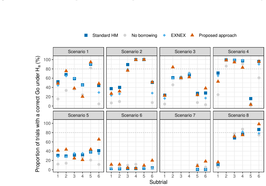
The central claim is that a distributional discrepancy, specifically the Hellinger distance between the posterior densities of the treatment effect in two subtrials, can serve as a direct measure of commensurability that governs information borrowing in a basket trial. The paper sets the spike-and-slab prior weight $w_{kk⋆}$ equal to the Hellinger distance $d_H(π_{θ_k}, π_{θ_{k⋆}})$: a distance near zero concentrates prior mass on the 'spike', so the complementary subtrial's data are essentially pooled in, while a distance near one concentrates mass on the 'slab', discarding the complementary data. For $K ≥ 3$ subtrials, the pairwise commensurate predictive priors are combined into a marginal predictive prior with weights $p_{kk⋆} = exp(−d_{kk⋆}/s_0)$ normalised across sources, so only the most commensurate subtrial(s) effectively contribute. Updating this marginal predictive prior with the contemporary subtrial's own data yields a robust posterior for Go/No-go decisions. Simulation results show improved precision and potentially improved power relative to no borrowing, standard hierarchical models, and EXNEX, together with the ability to identify the most commensurate source and to quantify how much each subtrial contributes.
Load-bearing premise
The load-bearing premise is that the Hellinger distance between two subtrials' estimated treatment-effect distributions is a faithful, well-calibrated probability that the subtrials should not share information; if sample-size imbalance or estimation noise distorts that distance, the trial borrows the wrong amount and the claimed gains in precision and power do not follow.
Editorial extensions
If this is right
- In a basket trial with at least three subtrials, the analysis identifies the most commensurate source subtrial(s) and assigns them the largest weight in the marginal predictive prior, so borrowing concentrates where the treatment effects genuinely match.
- Estimates of a subtrial's treatment effect gain precision (narrower credible intervals, lower MSE) whenever at least one complementary subtrial has a similar effect, while inconsistent subtrials contribute little or nothing.
- The method collapses to complete pooling when all pairwise Hellinger distances are zero and to no borrowing when they are near one, recovering both conventional extremes as special cases.
- The same Hellinger-distance-weighted borrowing scheme can be applied to binary endpoints or other generalised linear models after fitting per-subtrial regressions, extending the approach beyond continuous endpoints.
- In mixed-null and global-null scenarios, the method's analogue of the type I error rate stays well below the no-borrowing approach under the global null and below the hierarchical and EXNEX alternatives when non-null subtrials have large effects, because sharing is limited to commensurate subtrials.
Reading between the lines
- The Hellinger distance is treated as a calibrated probability without propagating its own estimation uncertainty into the posterior; a calibration study regressing true effect differences on the derived weights across sample-size configurations would show how much miscalibration remains, especially when one subtrial is much larger than another.
- The tuning constant $s_0$ acts as a temperature for the weight transformation: a principled choice could be derived by targeting a desired error-rate ceiling or a minimum power gain instead of being fixed at 0.15.
- The same discrepancy-weighted borrowing idea transfers naturally to umbrella or platform trials whose arms open asynchronously, where the 'most commensurate source' could be re-selected adaptively as data accumulate, connecting this work to dynamic borrowing in sequential designs.
- The method's Go/No-go criterion can be tracked against the borrowing weights in interim analyses, giving a direct way to quantify how information sharing interacts with repeated-look type I error inflation.
Signed reviews
Editorial analysis
A structured set of objections, weighed in public.
Referee Report
Summary. This paper develops a Bayesian methodology for borrowing information across patient subgroups in randomised, placebo-controlled basket trials with a continuous endpoint. After covariate adjustment via linear regression, the evidence from each subtrial is summarised by an 'operational posterior.' The Hellinger distance d_H between the operational posteriors of two subtrials is used as (i) the prior probability w_{kk*} with which a spike-and-slab prior on the precision parameter of a commensurate predictive prior is in the discounting 'slab' component (Eqs. (5)-(6)), and (ii), for K >= 3, as the input to a softmax-type transform producing combination weights p_{kk*} (Eq. (11)) that merge the (K-1) commensurate predictive priors into a normal marginal predictive prior (Eqs. (8)-(9)), which is then updated with the contemporary subtrial data (Eq. (10)). Operating characteristics are assessed by simulation under nine scenarios with K = 6 subtrials of unequal sample sizes and 10,000 replicates, comparing the proposed method with a standard hierarchical model, a no-borrowing analysis, and the EXNEX model on bias, MSE, credible interval width, an analogue of type I error, and an analogue of power. The authors report lower bias and MSE in most scenarios, narrower credible intervals when consistent sources exist, higher power in several scenarios, and the ability to up-weight the most commensurate source; type I error results are reported honestly.
Significance. The problem is timely and the central idea, letting a distributional discrepancy measure govern the amount of borrowing without assuming exchangeability, is attractive. If fully established, the contribution would be useful: it extends commensurate-prior borrowing to non-oncology basket trials with continuous endpoints, uses a symmetric and transformation-invariant measure, handles K >= 3 by differential weighting, and is accompanied by reproducible code and a carefully designed simulation study (nine scenarios, 10,000 replicates, including mixed-null and global-null cases). The supplementary sensitivity analyses for the tuning scale s0 and for unequal sample sizes are additional strengths, as is the explicit acknowledgment that the slab component of the spike-and-slab prior is not calibrated. However, the load-bearing calibration step w = d_H is not justified, the data are used twice in constructing the prior, and an approximation in forming the marginal predictive prior is unexamined, as detailed below. These issues must be addressed before the precision and power claims can be accepted; the manuscript is therefore of genuine interest but not yet in publishable form.
major comments (3)
- [Section 3, Eqs. (5)-(6)] The stipulation w_{kk*} = d_H(π_{θ_k}, π_{θ_{k*}}) treats a plug-in Hellinger distance between finite-sample operational posteriors as the prior probability of incommensurability. With the essentially flat operational prior N(0, 10^2) used here, the posterior variance v is close to the sampling variance of the treatment-effect estimate, and the difference between two independent posterior means under equal true effects has variance 2v; the exponent in the Hellinger integrand then has mean 1/4, so the expected d_H under perfect consistency is around 0.4, essentially independent of n for pairs with comparable sample sizes, and larger still when posterior variances differ (for the paper's settings, v is about 0.064 at n = 10, σ = 0.4). The spike mass 1 - w_{kk*} is thus systematically well below 1 when subtrials are truly consistent, the convergence to complete pooling asserted in the note after Eq. (11) is a probability-zero idealisation, and the method borrows less than intended in the situations where borrowing is most valuable. Conversely, for genuinely discrepant effects the finite-sample noise compresses d_H for small subtrials. No calibration of the w = d_H mapping, no null-distribution analysis, and no propagation of the estimation uncertainty in d_H are provided; Supplementary Section D only illustrates two K = 2 datasets and does not quantify the sampling distribution of d_H. The Discussion's remark that the slab prior is not calibrated is welcome but does not cover this more consequential calibration. Because w_{kk*} and p_{kk*} set the amount of borrowing, the precision and power gains reported in Section 4.2 are not yet supported.
- [Section 3, Eqs. (6), (10)-(11)] The marginal predictive prior for θ_{k*} depends on the contemporary data through the Hellinger distance d_{kk*} = d_H(π(θ_k|x_k), π(θ_{k*}|x_{k*})), which enters both w_{kk*} in Eq. (5) and p_{kk*} in Eq. (11); the notation π_MPP(θ_{k*}|x_{(-k*)}) is therefore misleading because the 'prior' is a function of x_{k*} itself. Eq. (10) then multiplies this data-dependent prior by the likelihood L(x_{k*}|θ_{k*}), using x_{k*} twice. The resulting object is not a proper Bayesian posterior, and the manuscript does not flag this plug-in or empirical-Bayes aspect. The credible-interval widths and MSE values in Section 4.2 and in Figures 1 and S2 are valid frequentist summaries of a well-defined procedure, but interpreting the narrower intervals as a Bayesian gain is not justified, and the double use could plausibly inflate the apparent precision advantage. The authors should either reframe the method explicitly as empirical Bayes or quantify the effect of the double use, for example by comparing with a version in which d_{kk*} is computed from the complementary data alone plus a held-out portion of x_{k*}.
- [Section 3, Eqs. (7)-(9)] The marginal CPP in Eq. (7) is a scale mixture over the operational posterior of θ_k and the spike-and-slab prior on ν_{kk*}, so it is not exactly normal; the statement that it 'may be represented as a N(λ_k, ξ_k^2) distribution for the ease of notations' is an unexamined approximation, with no moment-matching calculation or error assessment. Relatedly, the synthesis of the (K-1) sources as a weighted sum of independent normals in Eq. (8), with variance Σ_k p^2_{kk*} ξ_k^2, is one of several possible ways to combine predictive priors (a mixture or product combination would behave differently), and no argument establishes that the convolution form is the appropriate one. The adequacy of both the normality approximation and the weighted-sum combination should be demonstrated, at least in a simple K = 3 example against the exact predictive distribution, because the resulting MPP is the prior that drives the posterior inference in Eq. (10).
minor comments (7)
- [Abstract / Section 1] The claim that 'only information from subtrial(s) with the most commensurate treatment effect is leveraged' overstates the method, since every p_{kk*} in Eq. (11) is strictly positive and every complementary subtrial therefore contributes, however slightly, to the marginal predictive prior in Eq. (8); 'predominantly' would be accurate, and the rest of the text indeed describes down-weighting rather than elimination.
- [Section 4.2] The credible-interval comparison is referenced as 'Figure S1 of the Supplementary Materials,' but the relevant figure is S2; Figure S1 displays the prior density of the CPP standard deviation under the slab prior.
- [Table 1] The sample-size labels in the column headers ('2 (n3 = 10)', '3 (n2 = 14)', '4 (n5 = 16)', '5 (n4 = 20)') do not match the order n_k in {10, 10, 14, 16, 20, 20} stated in Section 4.1, making the scenario table hard to read; please correct the labels and keep the subtrial numbering consistent throughout.
- [Section 3, Eq. (5)] The spike-and-slab prior is defined only through its CDF; writing the mixture explicitly as g_k(ν) = w_{kk*}/(B2 - B1) on [B1, B2] plus a point mass (1 - w_{kk*}) at ν = S would be clearer and would remove the ambiguity concerning the behaviour of the distribution on (B2, S).
- [Section 4.1] The choice s0 = 0.15 is motivated only as 'to leverage information from all other subtrials'; the sensitivity analysis in Supplementary Section C examines the effect of s0 on the allocated weights but not on downstream operating characteristics (MSE, power, type I error), so how the headline conclusions depend on this tuning parameter remains unclear.
- [Supplementary Section D] The reported Hellinger distances appear inconsistent with the stated operational posteriors. For the σ = 0.4 unequal-size example, the posteriors are given as N(0.762, 0.19^2) and N(0.863, 0.05^2); the Hellinger distance between these two normal densities is approximately 0.59, not the reported 0.08, whether 0.19 and 0.05 are read as standard deviations or as variances. The σ = 0.8 examples likewise report 0.16 where the stated densities give distances of about 0.03 and 0.61. The illustration should be recomputed or the parameter values clarified.
- [Throughout] Several typos should be corrected, including 'dφH' after Eq. (6) (should be d_H), 'contemparory' in Section 1 (should be 'contemporary'), and 'accroding' in Supplementary Section C (should be 'according').
Circularity Check
The borrowing weight is fitted from the same subtrial data it then summarizes, so the claimed precision/power gains are partly in-sample double use.
-
fitted input called prediction
[Section 3, Eqs. (5), (6), (10)]
"We may then relate the ‘slab’ prior probability wkk⋆ with the computed Hellinger distance, simply by stipulating wkk⋆ = dH(πθk,πθk⋆). ... πMPP(θk⋆|xk⋆, x(−k⋆))∝L(xk⋆|θk⋆)×πMPP(θk⋆|x(−k⋆))."
The Hellinger distance in Eq. (6) is computed from the operational posteriors πk(θk|xk) and πk⋆(θk⋆|xk⋆), so it is a function of the contemporary subtrial data xk⋆. That same distance is stipulated as wkk⋆ in Eq. (5), governing how much information is borrowed through the commensurate predictive prior, and is then transformed in Eq. (11) into the weights pkk⋆ that define the marginal predictive prior used in Eq. (10). Equation (10) multiplies this data-dependent prior by the likelihood L(xk⋆|θk⋆) for the very same data xk⋆. Hence the amount of borrowing is fitted to the data it then acts on, and the current subtrial's data enter the final posterior twice: once through the distance-derived prior and once through the likelihood.
full rationale
The core derivation chain is self-contained in the sense that the methodology is not justified by a self-citation chain: the commensurate-prior framework is cited from Hobbs et al. but the present paper's contribution is the Hellinger-distance-based weight construction, which is new and independently checkable. However, a genuine circularity arises within the paper's own equations: the borrowing weight w_{kk*} and the combination weights p_{kk*} are computed from the same subtrial data that are subsequently used as the likelihood in the final posterior update. This is not merely a statistical opinion; it follows directly from Eq. (6) (distance from posterior densities that include x_{k*}), Eq. (5) (w = d_H), Eq. (11) (p from d_H), and Eq. (10) (same x_{k*} in the likelihood). The paper acknowledges the dependence on sample size in Supplementary Section D but does not quantify the null distribution or calibrate the mapping, so the claimed precision and power gains in Section 4.2 are inflated by this double use. This is a fitted-input-as-prediction pattern, not a self-citation problem. Given that the central mechanism reduces to a data-driven prior constructed from the data it summarizes, a score of 6 is appropriate: the prediction of improved performance is partially forced by the construction, though the method still has independent content as an adaptive borrowing device.
Assumptions & free parameters
free parameters (3)
- s0 (weight transformation scale) =
0.15 (simulation default; sensitivity explored at 0.25, 0.35, 0.45)
- B1, B2, S (spike-and-slab prior limits) =
0.01, 1, 100
- Half-normal prior scale for covariate random effects =
1
assumptions (6)
- domain assumption The linear regression model (1) correctly specifies the outcome distribution within each subtrial.
- domain assumption The commensurate predictive prior with normal form N(θk, 1/ν²) adequately captures the relationship between subtrial treatment effects.
- domain assumption The spike-and-slab prior form in Eq. (5) is appropriate for the precision parameter ν.
- ad hoc to paper The Hellinger distance between operational posteriors is a valid measure of the prior probability of incommensurability, so w = dH.
- ad hoc to paper The weight transformation Eq. (11) with softmax form and chosen s0 yields an appropriate combination of complementary CPPs.
- ad hoc to paper The combination of (K-1) CPPs into a single normal MPP via the weighted sum in Eqs. (8)-(9) is an adequate approximation to the true predictive distribution.
Cite this review
Pith. "Pith review of Borrowing of information across patient subgroups in a basket trial based on distributional discrepancy." pith.science (2026). https://pith.science/paper/NSIQBHSL
@misc{pith2026190805091,
  author       = {Pith},
  title        = {Pith review of: Borrowing of information across patient subgroups in a basket trial based on distributional discrepancy},
  year         = {2026},
  howpublished = {\url{https://pith.science/paper/NSIQBHSL}},
  note         = {Machine review of arXiv:1908.05091}
}
read the original abstract
Basket trials have emerged as a new class of efficient approaches in oncology to evaluate a new treatment in several patient subgroups simultaneously. In this paper, we extend the key ideas to disease areas outside of oncology, developing a robust Bayesian methodology for randomised, placebo-controlled basket trials with a continuous endpoint to enable borrowing of information across subtrials with similar treatment effects. After adjusting for covariates, information from a complementary subtrial can be represented into a commensurate prior for the parameter that underpins the subtrial under consideration. We propose using distributional discrepancy to characterise the commensurability between subtrials for appropriate borrowing of information through a spike-and-slab prior, which is placed on the prior precision factor. When the basket trial has at least three subtrials, commensurate priors for point-to-point borrowing are combined into a marginal predictive prior, according to the weights transformed from the pairwise discrepancy measures. In this way, only information from subtrial(s) with the most commensurate treatment effect is leveraged. The marginal predictive prior is updated to a robust posterior by the contemporary subtrial data to inform decision making. Operating characteristics of the proposed methodology are evaluated through simulations motivated by a real basket trial in chronic diseases. The proposed methodology has advantages compared to other selected Bayesian analysis models, for (i) identifying the most commensurate source of information, and (ii) gauging the degree of borrowing from specific subtrials. Numerical results also suggest that our methodology can improve the precision of estimates and, potentially, the statistical power for hypothesis testing.
Figures

Reference graph
Works this paper leans on
-
[1]
Bernardo, J. (1996). The concept of exchangeability and its applications. Far East Journal of Mathematical Sciences , 4:111--122
work page 1996
-
[2]
Berry, S., Broglio, K., Groshen, S., and Berry, D. (2013). Bayesian hierarchical modeling of patient subpopulations: Efficient designs of phase II oncology clinical trials. Clinical Trials , 10:720--734
work page 2013
-
[3]
Bryant, J. and Day, R. (1995). Incorporating toxicity considerations into the design of two-stage phase II clinical trials. Biometrics , 51:1372--1383
work page 1995
-
[4]
Chu, Y. and Yuan, Y. (2018). A Bayesian basket trial design using a calibrated Bayesian hierarchical model. Clinical Trials , 15:149--158
work page 2018
-
[5]
Cunanan, K., Iasonos, A., Shen, R., Begg, C., and G \"o nen, M. (2017). An efficient basket trial design. Statistics in Medicine , 36:1568--1579
work page 2017
-
[6]
Cunanan, K., Iasonos, A., Shen, R., and G \"o nen, M. (2019). Variance prior specification for a basket trial design using bayesian hierarchical modeling. Clinical Trials , 16:142--153
work page 2019
-
[7]
Dey, D. and Birmiwal, L. (1994). Robust Bayesian analysis using divergence measures. Statistics & Probability Letters , 20:287 -- 294
work page 1994
-
[8]
Draper, D. (1995). Assessment and propagation of model uncertainty. Journal of the Royal Statistical Society. Series B (Methodological) , 57:45--97
work page 1995
Show all 36 references
-
[9]
Eisenhauer, E., Therasse, P., and Bogaerts, J. et al. . (2009). New response evaluation criteria in solid tumours: Revised recist guideline (version 1.1). European Journal of Cancer , 45:228 -- 247
2009
-
[10]
Multiple Endpoints in Clinical Trials
FDA (2017). Multiple Endpoints in Clinical Trials . US Food and Drug Administration: Rockville, MD
2017
-
[11]
Hobbs, B., Carlin, B., Mandrekar, S., and Sargent, D. (2011). Hierarchical commensurate and power prior models for adaptive incorporation of historical information in clinical trials. Biometrics , 67:1047--1056
2011
-
[12]
Hobbs, B., Carlin, B., and Sargent, D. (2013). Adaptive adjustment of the randomization ratio using historical control data. Clinical Trials , 10:430--440
2013
-
[13]
and Landin, R
Hobbs, B. and Landin, R. (2018). Bayesian basket trial design with exchangeability monitoring. Statistics in Medicine , 37:3557--3572
2018
-
[14]
Hobbs, B., Sargent, D., and Carlin, B. (2012). Commensurate priors for incorporating historical information in clinical trials using general and generalized linear models. Bayesian Analysis , 7:639--674
2012
-
[15]
Hyman, D., Piha-Paul, S., and Won, H. et al. . (2018). HER kinase inhibition in patients with HER2- and HER3-mutant cancers. Nature , 554:189--194
2018
-
[16]
Hyman, D., Puzanov, I., and Subbiah, V. et al. . (2015). Vemurafenib in multiple nonmelanoma cancers with BRAF V600 mutations. New England Journal of Medicine , 373:726--736
2015
-
[17]
Jeffreys, H. (1961). Theory of Probability . Oxford University Press: Amen House, London
1961
-
[18]
Liu, R., Liu, Z., Ghadessi, M., and Vonk, R. (2017). Increasing the efficiency of oncology basket trials using a Bayesian approach. Contemporary Clinical Trials , 63:67 -- 72
2017
-
[19]
and Raftery, A
Madigan, D. and Raftery, A. (1994). Model selection and accounting for model uncertainty in graphical models using Occam's window. Journal of the American Statistical Association , 89:1535--1546
1994
-
[20]
Mirnezami, R., Nicholson, J., and Darzi, A. (2012). Preparing for precision medicine. New England Journal of Medicine , 366:489--491
2012
-
[21]
and Beauchamp, J
Mitchell, T. and Beauchamp, J. (1988). Bayesian variable selection in linear regression. Journal of the American Statistical Association , 83:1023--1032
1988
-
[22]
Mutsvari, T., Tytgat, D., and Walley, R. (2016). Addressing potential prior-data conflict when using informative priors in proof-of-concept studies. Pharmaceutical Statistics , 15:28--36
2016
-
[23]
Neuenschwander, B., Wandel, S., Roychoudhury, S., and Bailey, S. (2016). Robust exchangeability designs for early phase clinical trials with multiple strata. Pharmaceutical Statistics , 15:123--134
2016
-
[24]
Pardo, L. (2005). Statistical Inference Based on Divergence Measures . Statistics: A Series of Textbooks and Monographs. CRC Press
2005
-
[25]
Psioda, M., Xu, J., Jiang, Q., Ke, C., Yang, Z., and Ibrahim, J. (2019). Bayesian adaptive basket trial design using model averaging . Biostatistics . Epub ahead of print
2019
-
[26]
and Mandrekar, S
Renfro, L. and Mandrekar, S. (2018). Definitions and statistical properties of master protocols for personalized medicine in oncology. Journal of Biopharmaceutical Statistics , 28:217--228
2018
-
[27]
and Sargent, D
Renfro, L. and Sargent, D. (2017). Statistical controversies in clinical research: basket trials, umbrella trials, and other master protocols: a review and examples. Annals of Oncology , 28:34--43
2017
-
[28]
Schork, N. (2015). Personalized medicine: Time for one-person trials. Nature , 520:609--611
2015
-
[29]
Schwartz, L., Liti\` e re, S., and de Vries, E. et al. . (2016). Recist 1.1 -- update and clarification: From the recist committee. European Journal of Cancer , 62:132 -- 137
2016
-
[30]
Simon, R., Geyer, S., Subramanian, J., and Roychowdhury, S. (2016). The bayesian basket design for genomic variant-driven phase ii trials. Seminars in Oncology , 43:13 -- 18
2016
-
[31]
Spiegelhalter, D., Freedman, L., and Parmar, M. (1994). Bayesian approaches to randomized trials. Journal of the Royal Statistical Society. Series A (Statistics in Society) , 157:357--416
1994
-
[32]
and Wathen, J
Thall, P. and Wathen, J. (2008). Bayesian designs to account for patient heterogeneity in phase II clinical trials. Current Opinion in Oncology , 20:407—411
2008
-
[33]
Thall, P., Wathen, J., Bekele, B., Champlin, R., Baker, L., and Benjamin, R. (2003). Hierarchical Bayesian approaches to phase II trials in diseases with multiple subtypes. Statistics in Medicine , 22:763--780
2003
-
[34]
Tournoux, C., Rycke, Y., M \'e dioni, J., and Asselain, B. (2007). Methods of joint evaluation of efficacy and toxicity in phase II clinical trials. Contemporary Clinical Trials , 28:514 -- 524
2007
-
[35]
and LaVange, L
Woodcock, J. and LaVange, L. (2017). Master protocols to study multiple therapies, multiple diseases, or both. New England Journal of Medicine , 377:62--70
2017
-
[36]
Zheng, H., Hampson, L., and Wandel, S. (2020). A robust Bayesian meta-analytic approach to incorporate animal data into phase I oncology trials. Statistical Methods in Medical Research , 29:94--110
2020
Reviewed August 14, 2026 · model on record in the stance chip above.
Discussion (0). Continue with ORCID to comment.