REVIEW 2 major objections 4 minor 45 references
Computation of conformal invariants
T0 review · 2 major / 4 minor · reviewed 2026-08-14 · deepseek-v4-flash
Pith's one-line read One integral solver computes conformal capacity to 14 digits.
desk verdict A solid, well-validated computational paper; the elliptic-capacity conjugate worry does not survive reading, but the non-symmetric benchmark could be tightened. read the letter →
The pith
A machine-rendered reading of the paper's core claim, the machinery that carries it, and where it could break.
The reading
What carries the argument
The central object is the generalized Neumann kernel $N(s,t)$, a continuous kernel built from the boundary parametrization and an auxiliary function $A$; with its singular companion $M(s,t)$ it forms the integral equation $(I-N)\rho=-M\gamma$, which is uniquely solvable. The load-bearing identity is $q=e^{h_2-h_1}$, where $h_1,h_2$ are the two values of the piecewise constant function $h=[M\rho-(I-N)\gamma]/2$ on the two boundary components. This identity turns the numerical solution of a linear integral equation into the modulus of the annulus conformally equivalent to the given domain, and therefore into the capacity $2\pi/\log(1/q)$. The paper packages that whole computation in one function, `annq`, whose output feeds every example in the text.
What would settle it
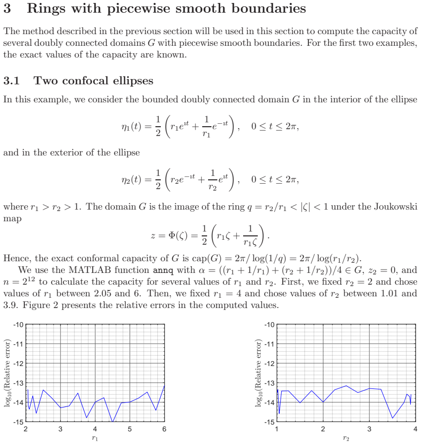
Use the confocal-ellipse ring with $r_1>r_2>1$, for which the exact capacity is $2\pi/\log(r_1/r_2)$; with $r_2=2$, $r_1=4$, and $n=2^{12}$ discretization points per boundary, the method should give a relative error near $10^{-14}$. If it does not, the claimed smooth-boundary accuracy fails.
Extended reading notes
Core claim
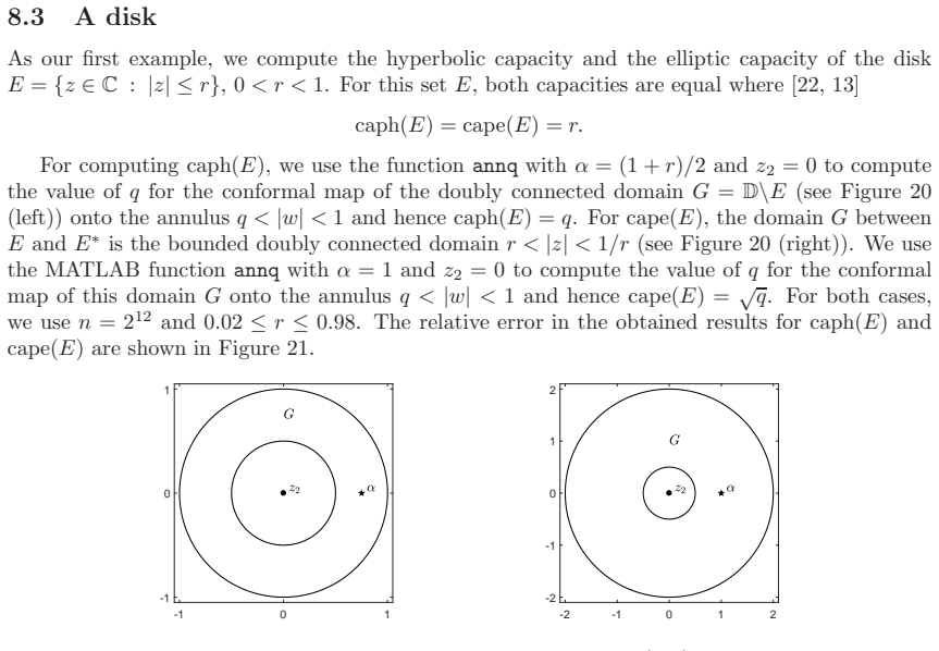
The paper establishes that the conformal capacity, hyperbolic capacity, and elliptic capacity of planar domains can all be extracted from a single computation: the conformal modulus $q$ of an associated doubly connected domain. Solving the generalized Neumann kernel integral equation on the two boundary curves yields a piecewise constant function $h$, and the identity $q=e^{h_2-h_1}$ gives the modulus of the annulus to which the domain maps; conformal invariance then forces $\mathrm{cap}(G)=2\pi/\log(1/q)$. For a compact connected set $E\subset\mathbb{D}$, the same $q$ with $G=\mathbb{D}\setminus E$ is the hyperbolic capacity, and with $G$ the region between $E$ and its antipodal set $E^*$, $\sqrt{q}$ is the elliptic capacity. Slit and half-plane boundaries are reduced to smooth rings by elementary maps or an iterative pre-mapping, and the same solver applies. Exact-formula comparisons show relative errors near $10^{-14}$ for smooth boundaries, and for cornered boundaries the values match known benchmarks to several digits.
Load-bearing premise
For slit and half-plane geometries, the capacity result relies on an auxiliary numerical pre-mapping that converts the slit into a smooth curve, and the paper does not analyze that pre-mapping's error.
Editorial extensions
If this is right
- A new doubly connected geometry needs only a boundary parametrization; the same solver returns its capacity, hyperbolic capacity, or elliptic capacity without a new derivation.
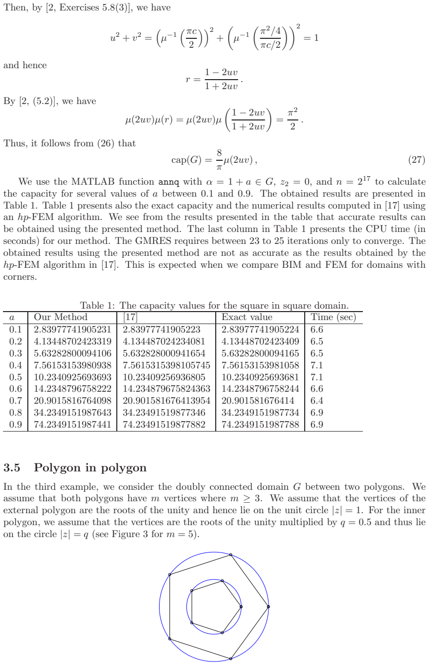
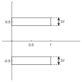
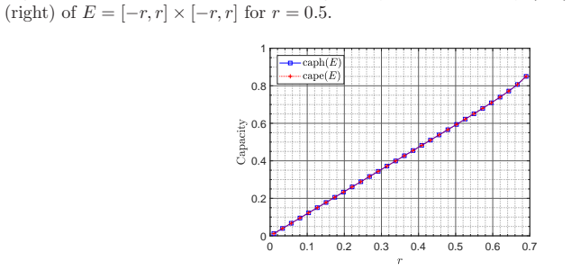
- For cornered geometries such as square-in-square, polygon-in-polygon, and rectangle-slits, the method produces stable values that in the tested tables match exact or benchmark values to several digits, so it can be used as a cross-check for other numerical schemes.
- The $O(n \log n)$ cost and reported runtimes below roughly ten seconds make parameter studies feasible, such as tracing capacity as a slit moves or as a boundary component changes shape.
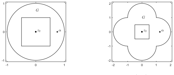
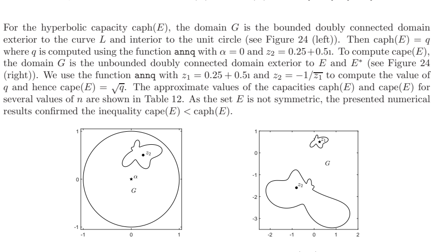
- The inequality $\mathrm{cap_e}(E)\le \mathrm{cap_h}(E)$ for compact connected subsets of the unit disk becomes numerically checkable for arbitrary shapes, as demonstrated for the non-symmetric amoeba region.
Reading between the lines
- Since several other conformal invariants, such as extremal length and moduli of curve families in doubly connected domains, are also functions of the annulus modulus $q$, the same computed $q$ could supply those values with no additional integral solving.
- A graded-mesh version of the trapezoidal rule, which the paper notes is needed at corners, should close the accuracy gap seen for square and polygon boundaries while keeping the same pipeline.
- The unquantified pre-mapping error for slit domains could be measured empirically by comparing the iterative pre-mapping results with the exact formulas for two-real-slits or half-plane slits.
- Because geometry enters only through the boundary parametrization, coupling the solver with automatic differentiation could produce geometric gradients of capacity, enabling shape optimization.
Signed reviews
Editorial analysis
A structured set of objections, weighed in public.
Referee Report
Summary. The paper presents a boundary integral equation method, based on the generalized Neumann kernel, for computing the conformal capacity of doubly connected planar domains by numerically constructing the conformal map onto a circular annulus. The authors supply a MATLAB implementation, annq, and validate it against exact formulas for several model geometries: two confocal ellipses, a square-in-square domain, two collinear slits, a segment and a circle, and a half-plane with a vertical slit. They report relative errors around 1e-14 for smooth boundaries and roughly twelve correct digits for corner domains. The method is then applied to slit and polygon geometries and to the numerical computation of hyperbolic and elliptic capacities of compact sets in the unit disk.
Significance. If the advertised claims are fully supported, the paper provides a useful, versatile, and easily modifiable computational tool for conformal invariants. Its strengths are the independent exact-formula benchmarks, the explicit MATLAB code, and the fact that the reported errors are not fitted to the benchmarks. The ring-capacity and hyperbolic-capacity results are convincing. However, the elliptic-capacity branch, which is part of the advertised scope, is currently undermined by an incorrect definition of the antipodal set in Section 8.2 and by a consequently invalid numerical test in Section 8.5. The central computational method itself appears sound, and the defect is localized and fixable.
major comments (2)
- [Section 8.2, Eqs. (47)-(48), and Section 8.5, Table 12] The definition of the antipodal set E* = {-1/a : a in E} is not the involution used in the Duren-Kuhnau elliptic capacity theory cited as [13]. The elliptic capacity of a set in the disk is associated with the fixed-point-free anti-Mobius antipodal map a -> -1/\bar a; the map a -> -1/a printed in the paper is a different holomorphic involution with fixed points ±i, and the two definitions agree only for sets invariant under complex conjugation. As a consequence, for the non-conjugation-symmetric amoeba of Section 8.5 the doubly connected domain between E and the incorrectly defined E* is not the annulus whose modulus yields cape(E), and the values labeled cape(E) in Table 12 together with the reported numerical confirmation of cape(E) < caph(E) do not test the stated inequality. The definition also breaks down when 0 belongs to E. Please replace E* by {-1/\bar a : a in E}, interpreted on the Riemann sphere when needed, recompute Section 8.5, and ensure that the code underlying annq uses the corrected definition.
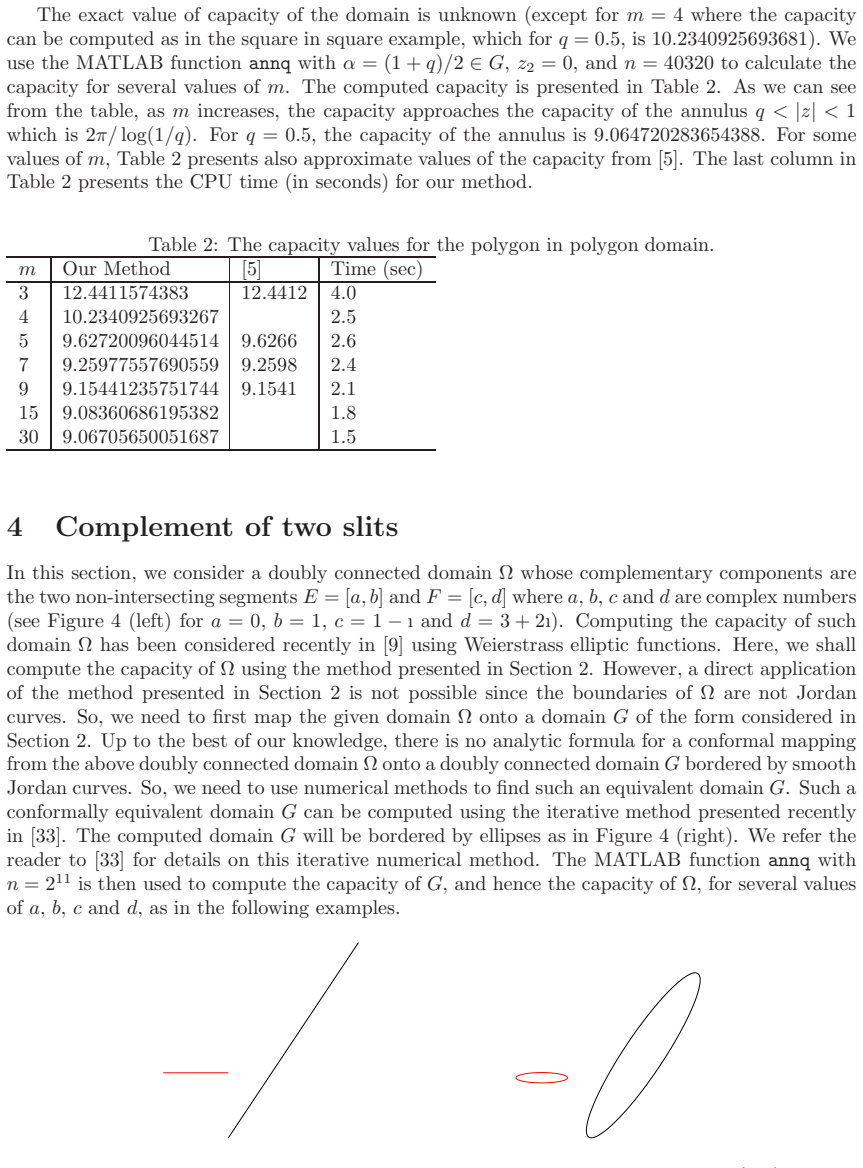
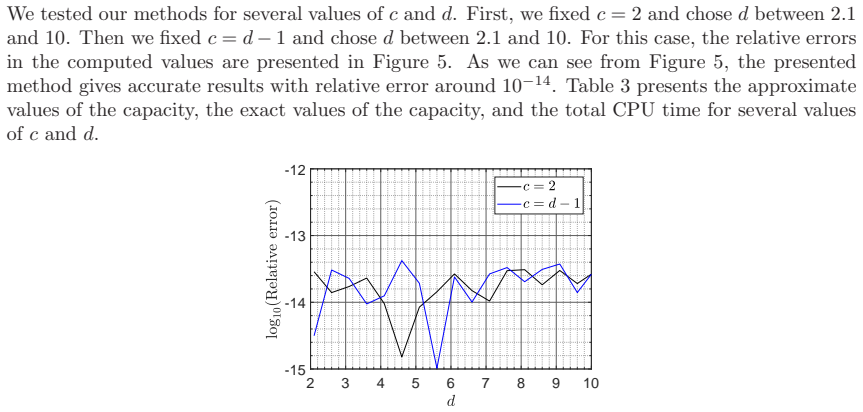
- [Sections 4 and 6] The general two-slit and half-plane-with-slit computations rely on the iterative method of [33] to construct a smooth doubly connected model domain, but the paper does not analyze the convergence or the accuracy of this auxiliary step. The benchmarks in Sections 4.1 and 6 with exact formulas show that the composed method is accurate in those cases, including the iterative step; however, for the genuinely non-symmetric configurations in Section 4.3 and Figure 16 no error estimate or refinement study for the auxiliary mapping is supplied. Because the advertised scope includes slit geometries, the authors should either quantify the error introduced by this step, for example by varying the stopping criterion of the iteration or comparing successive iterates, or explicitly state that these specific results are benchmark-dependent.
minor comments (4)
- [Sections 2.3 and 7.3] There are several typographical errors: "using using MATLAB R2017a" in Section 2.3, "In view of of (7)" near Eq. (8), and "the the auxiliary map" in Section 7.3.
- [Section 8.3, Figure 21] The caption of Figure 21 mentions a quantity c(E) that is not defined in the text; it should be defined or removed.
- [Section 7.1, Table 9] The "exact" capacity at the bottom of Table 9 is itself obtained by numerically solving equations (43) with Mathematica; the reported agreement of 1.5e-9 is several orders of magnitude larger than the other errors in the paper, so the precision of the Mathematica solution and the source of this discrepancy should be stated.
- [Table 5] The header "z2\z1" is confusing because the row entries appear to be values of z2 while the columns are values of z1; the layout should be clarified.
Circularity Check
Derivation is self-contained: the BIE solver is validated against independent exact formulas, and no fitted quantity is renamed as a prediction.
full rationale
I find no circular step that reduces an output to an input by construction. The paper's capacity computation reduces to computing the modulus q of a doubly connected domain by solving the boundary integral equation (9) and applying q = exp(h2 - h1) and cap(G) = 2*pi/log(1/q). Theorems 1 and 2, quoted from the authors' earlier work [28], state that q is obtained from the solution of the integral equation; this is a mathematical reduction, not a fit: the functions h and rho are obtained by solving an operator equation, and the exact benchmark values (confocal ellipses via the Joukowski map, square-in-square via elliptic integrals, two real segments via [44], segment-circle via [44]) are independent formula evaluations, not values used to determine any parameter. No parameter is fitted to a subset of capacity data and then "predicted" on a closely related quantity. The self-citations [28]-[30] and [33] supply the numerical method, the fbie implementation, and the iterative auxiliary mapping; they are load-bearing in the sense that the implementation is reused, but they are published, externally testable methods and do not encode the benchmark capacities or the claimed numerical results. The hyperbolic- and elliptic-capacity sections invoke the external theorems of Duren and Kuhnau [13] relating caph(E) = q and cape(E) = sqrt(q) to moduli of auxiliary domains; these are used as theoretical inputs, not as circular definitions, since the transfinite-diameter definitions (45) and (47) are stated separately. The reported inequality cape(E) < caph(E) for the amoeba-shaped set is obtained from two independent BIE computations and is not imposed by any fitted parameter. The skeptical note about the antipodal set E* = {-1/a} omitting the complex conjugate, if correct, is a mathematical correctness concern about the elliptic-capacity example, not a circularity: it does not show that a claimed output is equivalent by construction to an input. Accordingly, no circular step with the required quote-and-reduction evidence is present, and the circularity score is 0.
Assumptions & free parameters
assumptions (5)
- standard math Every doubly connected domain (ring) can be conformally mapped onto an annulus {q < |z| < 1}.
- standard math The generalized Neumann kernel integral equation (I-N)rho = -M gamma is uniquely solvable and yields a piecewise constant h.
- standard math Capacity is invariant under conformal mappings.
- domain assumption For slit and half-plane domains, the iterative method [33] produces a conformally equivalent domain bordered by smooth Jordan curves.
- standard math Hyperbolic capacity caph(E) equals q and elliptic capacity cape(E) equals sqrt(q) for a domain whose conformal modulus is q.
Cite this review
Pith. "Pith review of Computation of conformal invariants." pith.science (2026). https://pith.science/paper/O42JQVTI
@misc{pith2026190804533,
  author       = {Pith},
  title        = {Pith review of: Computation of conformal invariants},
  year         = {2026},
  howpublished = {\url{https://pith.science/paper/O42JQVTI}},
  note         = {Machine review of arXiv:1908.04533}
}
read the original abstract
We study numerical computation of conformal invariants of domains in the complex plane. In particular, we provide an algorithm for computing the conformal capacity of a condenser. The algorithm applies for wide kind of geometries: domains are assumed to have smooth or piecewise smooth boundaries. The method we use is based on the boundary integral equation method developed and implemented in [30]. A characteristic feature of this method is that, with small changes in the code, a wide spectrum of problems can be treated and we include code snippets within the text to indicate implementation details. We compare the performance and accuracy to previous results in the cases when numerical data is available and also in the case of several model problems where exact results are available.
Figures

Figures from the paper (21 more)




Reference graph
Works this paper leans on
-
[33]
M. Nasser and C. Green , A fast numerical method for ideal fluid flow in domains with multiple stirrers , Nonlinearity, 31 (2018), pp. 815–837
work page 2018
-
[13]
P. Duren and R. K ¨uhnau, Elliptic capacity and its distortion under conformal mappi ng, J. Anal. Math., 89 (2003), pp. 317–335
work page 2003
-
[1]
Ahlfors , Conformal Invariants , McGraw-Hill, New York, 1973
L. Ahlfors , Conformal Invariants , McGraw-Hill, New York, 1973
work page 1973
-
[2]
G. D. Anderson, M. K. V amanamurthy, and M. Vuorinen , Conformal Invariants, Inequalities and Quasiconformal Maps , John Wiley, New York, 1997
work page 1997
-
[3]
K. Atkinson, The Numerical Solution of Integral Equations of the Second K ind, Cambridge University Press, Cambridge, 1997
work page 1997
- [4]
-
[5]
D. Betsakos, K. Samuelsson, and M. Vuorinen , The computation of capacity of planar condensers, Publ. Inst. Math. (Beograd) (N.S.), 75 (2004), pp. 233–252
work page 2004
-
[6]
S. Bezrodnykh, A. Bogatyrev, S. Goreinov, O. Grigoriev, H. H akula, and M. Vuorinen , On capacity computation for symmetric polygonal condenser s, J. Comput. Appl. Math., 361 (2019), pp. 271–282
work page 2019
Show all 45 references
-
[7]
Bowman , Introduction to Elliptic Functions with Applications , English Universities Press Ltd., London, 1953
F. Bowman , Introduction to Elliptic Functions with Applications , English Universities Press Ltd., London, 1953
1953
-
[8]
Byrd and M
P. Byrd and M. D. Friedman , Handbook of elliptic integrals for engineers and scientist s. Second edition, revised., Springer-Verlag, Berlin, 1971
1971
-
[9]
Methods Funct
D.Dautova, S.Nasyrov, and M.Vuorinen , Conformal module of the exterior of two rec- tilinear slits , Comput. Methods Funct. Theory, (2020), p. arXiv:1908.02459
2020 arXiv
-
[10]
DeLillo, A
T. DeLillo, A. Elcrat, and E. Kropf , Calculation of resistances for multiply con- nected domains using Schwarz-Christoffel transformations , Comput. Methods Funct. Theory, 11 (2011), pp. 725–745
2011
-
[11]
Driscoll and L
T. Driscoll and L. Trefethen , Schwarz-Christoffel mapping , Cambridge University Press, Cambridge, 2002
2002
-
[12]
Dubinin , Condenser Capacities and Symmetrization in Geometric Func tion Theory , Springer, Basel, 2014
V. Dubinin , Condenser Capacities and Symmetrization in Geometric Func tion Theory , Springer, Basel, 2014
2014
-
[14]
Embree and L
M. Embree and L. Trefethen , Green’s functions for multiply connected domains via con- formal mapping , SIAM Rev., 41 (1999), pp. 745–761. 25
1999
-
[15]
Garnett and D
J. Garnett and D. Marshall , Harmonic measure , Cambridge University Press, Cam- bridge, 2008
2008
-
[16]
Greengard and Z
L. Greengard and Z. Gimbutas , FMMLIB2D: A MATLAB tool- box for fast multipole method in two dimensions , version 1.2. ed., 2012. http://www.cims.nyu.edu/cmcl/fmm2dlib/fmm2dlib.html. Accessed 1 Jan 2018
2012
-
[17]
Hakula, A
H. Hakula, A. Rasila, and M. Vuorinen , On moduli of rings and quadrilaterals: algo- rithms and experiments , SIAM J. Sci. Comput., 33 (2011), pp. 279–302
2011
-
[18]
, Computation of exterior moduli of quadrilaterals , Electron. Trans. Numer. Anal., 40 (2013), pp. 436–451
2013
-
[19]
, Conformal modulus on domains with strong singularities and cusps, Electron. Trans. Numer. Anal., 48 (2018), pp. 462–478
2018
-
[20]
Hariri, R
P. Hariri, R. Kl ´ en, and M. Vuorinen , Conformally Invariant Metrics and Quasiconfor- mal Mappings , Springer Monographs in Mathematics, Springer, Switzerland, 202 0
-
[21]
Keen and N
L. Keen and N. Lakic , Hyperbolic geometry from a local viewpoint , Cambridge University Press, Cambridge, 2007
2007
-
[22]
Kirsch , Transfinite diameter, Chebyshev constant and capacity , in Handbook of Complex Analysis: Geometric Function Theory, Vol
S. Kirsch , Transfinite diameter, Chebyshev constant and capacity , in Handbook of Complex Analysis: Geometric Function Theory, Vol. 2, R. K¨ uhnau, ed., Elsev ier, Amsterdam, 2005, pp. 243–308
2005
-
[23]
Kress , A Nystr¨ om method for boundary integral equations in domain s with corners , Nu- mer
R. Kress , A Nystr¨ om method for boundary integral equations in domain s with corners , Nu- mer. Math., 58 (1990), pp. 145–161
1990
-
[24]
, Linear Integral Equations , Springer, New York, 2014
2014
-
[25]
K ¨uhnau, ed
R. K ¨uhnau, ed. , Handbook of complex analysis: geometric function theory. V ol. 1, 2002, Vol. 2, 2005 , Elsevier Science B.V., Amsterdam
2002
-
[26]
Kythe , Handbook of conformal mappings and applications , Taylor & Francis Group, Boca Raton, 2019
P. Kythe , Handbook of conformal mappings and applications , Taylor & Francis Group, Boca Raton, 2019
2019
-
[27]
Liesen, O
J. Liesen, O. S ´ ete, and M. Nasser , Fast and accurate computation of the logarithmic capacity of compact sets , Comput. Methods Funct. Theory, 17 (2017), pp. 689–713
2017
-
[28]
Nasser , Numerical conformal mapping via a boundary integral equati on with the gener- alized Neumann kernel , SIAM J
M. Nasser , Numerical conformal mapping via a boundary integral equati on with the gener- alized Neumann kernel , SIAM J. Sci. Comput., 31 (2009), pp. 1695–1715
2009
-
[29]
, Numerical conformal mapping of multiply connected regions onto the second, third and fourth categories of Koebe canonical slit domains , J. Math. Anal. Appl., 382 (2011), pp. 47–56
2011
-
[30]
, Fast solution of boundary integral equations with the gener alized Neumann kernel , Elec- tron. Trans. Numer. Anal., 44 (2015), pp. 189–229
2015
-
[31]
, Numerical computing of preimage domains for bounded multip ly connected slit domains , J. Sci. Comput., 78 (2019), pp. 582–606
2019
-
[32]
Nasser and F
M. Nasser and F. Al-Shihri , A fast boundary integral equation method for conformal mapping of multiply connected regions , SIAM J. Sci. Comput., 33 (2013), pp. A1736–A1760
2013
-
[34]
Nasser, A
M. Nasser, A. Murid, and Z. Zamzamir , A boundary integral method for the Riemann- Hilbert problem in domains with corners , Complex Var. Elliptic Equ., 53 (2008), pp. 989–1008
2008
-
[35]
Nasser and M
M. Nasser and M. Vuorinen , Conformal invariants in simply connected domains , (2020), p. arXiv:2001.10182
2020 arXiv
-
[36]
, Numerical computation of the capacity of generalized conde nsers, J. Comput. Appl. Math., 377 (2020), p. 112865. 26
2020
-
[37]
Olver, D
F. Olver, D. Lozier, R. Boisvert, and C. W. Clark, eds. , NIST Handbook of Mathe- matical Functions, Cambridge University Press, Cambridge, 2010
2010
-
[38]
Papamichael and N
N. Papamichael and N. Stylianopoulos , Numerical conformal mapping: Domain de- composition and the mapping of quadrilaterals , World Scientific, New Jersey, 2010
2010
-
[39]
Saff and V
E. Saff and V. Totik , Logarithmic potentials with external fields , Springer-Verlag, Berlin, 1997
1997
-
[40]
Schinzinger and P
R. Schinzinger and P. Laura , Conformal mapping. Methods and applications , Dover Pub- lications, Inc., New York, 2003
2003
-
[41]
Trefethen and J
L. Trefethen and J. Weideman , The exponentially convergent trapezoidal rule , SIAM Review, 56 (2014), pp. 385–458
2014
-
[42]
V asil’ev, Moduli of Families of Curves for Conformal and Quasiconform al Mappings , Springer-Verlag, Berlin, 2002
A. V asil’ev, Moduli of Families of Curves for Conformal and Quasiconform al Mappings , Springer-Verlag, Berlin, 2002
2002
-
[43]
Vuorinen , Conformal invariants and quasiregular mappings , J
M. Vuorinen , Conformal invariants and quasiregular mappings , J. Anal. Math., 45 (1985), pp. 69–115
1985
-
[44]
Lecture Not es in Mathematics , Springer-Verlag, Berlin, 1988
, Conformal geometry and quasiregular mappings. Lecture Not es in Mathematics , Springer-Verlag, Berlin, 1988
1988
-
[45]
Wegmann and M
R. Wegmann and M. Nasser , The Riemann-Hilbert problem and the generalized Neumann kernel on multiply connected regions , J. Comput. Appl. Math., 214 (2008), pp. 36–57. 27
2008
Reviewed August 14, 2026 · model on record in the stance chip above.
Discussion (0). Continue with ORCID to comment.