Discontinuous Galerkin Semidiscretization of the Information Geometric Regularized Compressible Euler Equations

Brook Eyob; Florian Sch\"afer; Jesus Arias; Spencer H. Bryngelson

REVIEW 4 major objections 4 minor 1 cited by

Discontinuous Galerkin Semidiscretization of the Information Geometric Regularized Compressible Euler Equations

T0 review · 4 major / 4 minor · reviewed 2026-08-04 · deepseek-v4-flash

Challenge this review Re-run · record.json Download PDF Read on arXiv ↗ Review JSON

Pith's one-line read This paper claims that a discontinuous Galerkin discretization of information-geometric regularization stabilizes shocks in the compressible Euler equations without shock-capturing limiters or artificial viscosity, while preserving fine-sca

desk verdict A genuinely new DG realization of IGR with stable shocks on benchmarks, but the abstract's 'minimal activation' claim does not survive the paper's own convergence study. read the letter →

arxiv 2608.02223 v1 pith:O65GJWQB submitted 2026-08-03 math.NA cs.NA

Brook Eyob , Jesus Arias , Spencer H. Bryngelson , Florian Schäfer This is my paper · ORCID

classification math.NAcs.NA MSC 65M6076N1535L65

keywords discontinuousGalerkinshockcapturinginformationgeometricregularizationcompressibleEulerequationshyperbolic-ellipticsystemsentropicpressuresymmetricinteriorpenaltyhigh-ordermethods

verification ladder T0 review T1 audit T2 compute T3 formal

The pith

A machine-rendered reading of the paper's core claim, the machinery that carries it, and where it could break.

The reading

The paper develops a discontinuous Galerkin (DG) realization of information-geometric regularization (IGR) for the compressible Euler equations. The key idea is to regularize shocks at the PDE level by adding an entropic pressure Σ, obtained from an auxiliary elliptic equation, so that the Euler fluxes carry P+Σ instead of P alone. In numerical experiments, the resulting IGR-DG method stabilizes shocks without limiters or artificial viscosity, keeps Σ localized near compression, and retains fine-scale features better than a characteristic TVB-limited DG baseline, especially at higher polynomial order. If correct, this gives a genuinely inviscid, PDE-level alternative to dissipation-based shock capturing for high-order DG methods.

What carries the argument

The central object is the entropic pressure Σ, defined by the elliptic equation ρ⁻¹Σ − α∇·(ρ⁻¹∇Σ) = α[(tr Du)² + tr((Du)²)]. It is the mechanism that redistributes compression: it replaces the developing discontinuity with a smooth profile of width proportional to √α, without any viscous flux term. In the DG setting, Σ is computed by SIPG from the same polynomial space as the conserved variables, and enters the Euler equations only through the augmented pressure P+Σ in the momentum and energy fluxes; this preserves conservative structure and makes the elliptic solve the only global coupling beyond the elementwise numerical flux.

What would settle it

Run a smooth, non-shocking Euler flow (e.g., the nonlinear periodic simple wave of Example 1) on the same grid with the same polynomial order, comparing IGR-DG against unregularized DG with no limiter. If, before shock formation, the L1 error of IGR-DG does not approach that of the unregularized method under mesh refinement, then Σ is not minimal in smooth regions and the claim of selective activation fails directly.

Watch

Extended reading notes

Core claim

The central claim is that coupling a standard DG transport discretization (with a local Lax–Friedrichs flux) to a symmetric interior penalty Galerkin (SIPG) solve for the entropic pressure Σ yields stable shock resolution in Euler flows without any limiter or artificial viscosity. The regularization is defined by the elliptic equation ρ⁻¹Σ − α∇·(ρ⁻¹∇Σ) = α[(tr Du)² + tr((Du)²)], where α controls strength and the length scale over which compression is redistributed; the same polynomial space is used for both hyperbolic and elliptic variables, and Σ enters the Euler fluxes only through the augmented pressure P+Σ. The paper's benchmarks — shock formation, propagation, shock–shock and shock–vort

Load-bearing premise

The load-bearing premise is that the entropic pressure Σ remains negligible in smooth regions of the flow, so the regularization does not degrade the underlying high-order DG accuracy away from shocks; the paper's own pre-shock convergence data show the regularization measurably slows convergence in smooth flow, putting this premise at risk.

Editorial extensions

If this is right

If correct, high-order DG methods can resolve post-shock oscillations and fine-scale structures that limiter-based methods typically damp.
The method removes the need for explicit shock sensors or limiting procedures, replacing them with one elliptic solve per time step.
The formulation is conservative and uses a common approximation space, so it may transfer to other hyperbolic systems sharing the same conservative structure, such as magnetohydrodynamics.
The fixed-total-DOF p-refinement study suggests IGR-DG avoids the error growth with polynomial order seen in TVB-limited DG for shock-dominated flows.
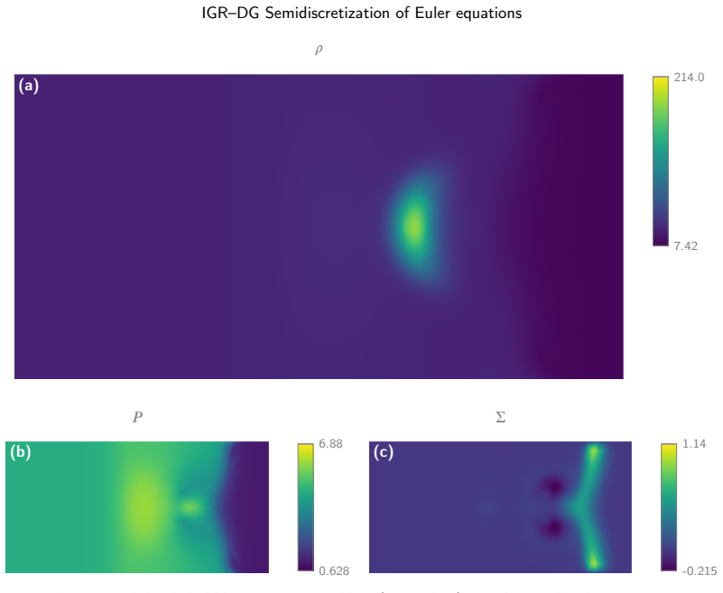
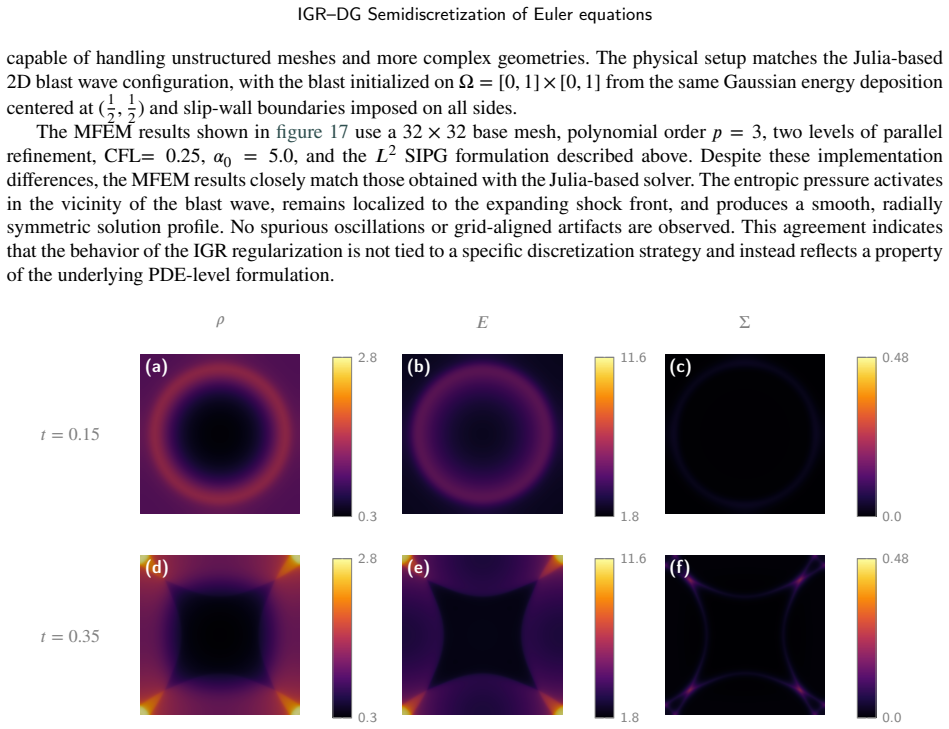
Multidimensional benchmarks show the regularization stays localized to the shock, preserving symmetry and avoiding grid-aligned artifacts.

Reading between the lines

Editorial extensions of the paper, not claims the author makes directly.

The paper's own Figure 2 shows that before a shock forms, IGR-DG converges at second order for p=3 versus fourth order for the limiter baseline; if this contamination is generic, the method trades smooth-flow accuracy for shock stability, and a scale- or sensor-dependent α would be needed to recover the full order.
The reported accuracy comparisons use fine-grid DG+limiter solutions as references for the smoothed Riemann problems, so the L1 errors measure agreement with the competing method rather than with an exact solution.
A predictive formula linking α to local compressive intensity would be needed to make the method parameter-free in practice; across the paper's tests α ranges from 0.3 to 32.
If the smooth-region contamination is confirmed, a natural testable extension is to apply Σ only to the high-wavenumber part of the velocity gradient, aiming to preserve formal accuracy while keeping shock stabilization.

Share X Bluesky LinkedIn Reddit HN

Editorial analysis

A structured set of objections, weighed in public.

Desk editor's note, referee report, and a circularity audit.

Desk Editor's Note

read the letter

The real contribution here is concrete: this is the first DG semidiscretization of the IGR-regularized Euler equations, coupling a DG Euler discretization with an SIPG solve for the entropic pressure in the same approximation space. The authors ship both Julia and MFEM code, and the benchmark suite is broad. The headline empirical result — stable shocks without limiters or artificial viscosity across 1D and 2D problems — is supported by the plots. The fixed-DOF p-refinement study is also genuinely informative: IGR-DG keeps error roughly flat as p increases, while the TVB limiter baseline gets worse. That is a real and useful observation.

The soft spots are real, though none are fatal. The abstract's "minimal activation in smooth regions" is contradicted by the paper's own Figure 2: pre-shock, p=3 IGR-DG converges at second order while DG+limiter converges at fourth order. Section 6 concedes this directly ("reduces the order of accuracy before shock formation"), so the paper is not hiding it — but the abstract overclaims, and the tension matters because the value proposition is precisely that the regularization preserves smooth flow. The per-problem tuning of alpha0 is a second weakness: the stability results show that a stabilizing parameter exists, not how to choose it without hand-fitting. The reference-solution methodology also biases the comparison, since errors are measured against fine-grid DG+limiter output; and the 2D experiments lack the baseline and error quantification that the abstract promises. None of these undercut the central stability result, but they do mean the paper is not yet the clean case for IGR-DG that the abstract suggests.

What the paper does well: it is honest about its own limitation in Section 6, it provides reproducible artifacts, and the MFEM independent implementation is a nice check that the behavior is not tied to one discretization framework. The math is coherent, and the method does what it claims on the tested benchmarks.

This paper deserves a serious referee. The right outcome is probably conditional acceptance after the abstract is toned down, the pre-shock accuracy loss is treated as a known tradeoff rather than an incidental detail, and the alpha-selection question is addressed head-on (even a sensitivity study would help). I would bring it to a reading group and cite it; the method is new enough and well-enough executed to be worth engaging with.

Referee Report

4 major / 4 minor

Summary. The paper proposes a discontinuous Galerkin (DG) discretization of the information-geometric regularization (IGR) of the compressible Euler equations. The entropic pressure Sigma is obtained from an auxiliary elliptic equation (Eq. 5), discretized with SIPG in the same DG space as the hyperbolic conservation law, and enters the Euler fluxes only through the augmented pressure P+Sigma (Eq. 7). The authors test the resulting IGR-DG method on one- and two-dimensional benchmarks, including shock formation, smoothed Riemann problems, Shu-Osher-type fine-scale problems, shock-bubble interaction, and a supersonic cylinder, comparing against a TVB-limited DG baseline. They claim shock stabilization without shock-capturing limiters or artificial viscosity, preservation of fine-scale features, and selective activation of Sigma concentrated in strongly compressive regions.

Significance. If the central claims hold, the paper would provide a useful PDE-level alternative to limiter- and viscosity-based shock capturing for high-order DG, with the practical advantage that the regularization is independent of mesh structure and polynomial order details. The availability of both a Julia implementation and an MFEM implementation is a strength and supports reproducibility. However, the significance is conditional on two load-bearing points: (i) the entropic pressure really is 'minimal' in smooth regions so that high-order accuracy is preserved, and (ii) the reported error comparisons are against trustworthy reference solutions. Both points are currently problematic, as detailed below.

major comments (4)

[Abstract, §2.1, Eq. (5), Fig. 2, §6] The abstract and §2.1 state that Sigma has 'minimal activation in smooth regions' and that the regularization preserves the underlying solution elsewhere. This is contradicted by the paper's own data. For any non-uniform velocity field, the right-hand side of Eq. (5) is nonzero, so at fixed alpha > 0 the entropic pressure is generically O(alpha) in smooth regions and enters the momentum and energy fluxes through Eq. (7). Figure 2 shows that, before shock formation in Example 1, IGR-DG at p=3 converges at only second order in density, momentum, and energy, while the DG+limiter baseline converges at fourth order. Section 6 explicitly concedes that 'IGR-DG reduces the order of accuracy before shock formation.' This is not a localized, negligible effect: it is a systematic modification of smooth flow. The claim of 'minimal activation' must be substantially revised or quantified, because it i
[§5.1, paragraph after Eq. (32); §5.1.3, Fig. 10] For all smoothed Riemann problems, the reference solutions are obtained from fine-grid DG+limiter simulations. Since the initial data are smoothed, the classical self-similar solutions are not exact, so the reported L1 errors measure the difference from the baseline method's output rather than from a physical/analytic solution. This is especially problematic in the modified Shu-Osher example, where the baseline is claimed to damp fine-scale oscillations: if the reference itself is smoothed, IGR-DG's lower 'error' may partly reflect a better match to the reference's smoothing, or a different kind of smoothing. Similarly, the p-refinement study in §5.1.3 uses an IGR-DG solution with m_ref=1024, p_ref=3, and alpha_0,ref=1.0 as the reference, which favors the method being compared. The quantitative convergence and error comparisons in Figs. 2, 4, 6, 8, and 9 need a more neutral reference, su
[§5.1.4, §5.1.3, parameter selection] The regularization strength alpha_0 is selected per problem to ensure stable evolution (e.g., 0.3 for the simple wave, 0.5 or 0.7 for Sod, 4.0 in the fixed-DOF Shu-Osher study, 32.0 for the shock-bubble case). Figure 12 provides only a p=1 threshold curve for a sinusoidal compressive wave and gives no predictive formula or criterion for choosing alpha_0 for a new problem. The claim in §5.1.4 that this provides a 'physically interpretable basis for parameter selection rather than ad hoc tuning' is not supported by the experiments. Furthermore, the p-refinement scaling alpha = alpha_0 h_eff^2 in §5.1.3, with h_eff = 2h/(p+1), is introduced without derivation or sensitivity study; the conclusion that IGR-DG has 'nearly constant error' across p may depend on this specific scaling and on the choice alpha_0=4.0. A method advertised as removing limiter-parameter tuning should come with a more p
[§5.2.2, Example 11, abstract/conclusion] The abstract says the method 'stabilizes shocks without shock-capturing limiters or artificial viscosity,' with a caveat that positivity-preserving methods may still be required. In the supersonic-cylinder example (Example 11), a Zhang-Shu positivity-preserving limiter is enabled. This is not necessarily a logical contradiction, since the limiter is not a shock-capturing limiter, but the central comparison in the conclusion says 'without shock-capturing limiters' rather than 'without any limiter.' The role of the positivity limiter in the benchmark suite should be stated clearly in the summary and conclusion so that readers do not infer limiters are absent in all tested configurations.

minor comments (4)

[§4.2, Eq. (23)] The local Lax-Friedrichs coefficient is written as lambda = (|u_n^-|+c^-, |u_n^+|+c^+), which looks like a pair rather than the expected maximum of the two local speeds. Please clarify the notation.
[Fig. 3/4 and Fig. 7/8] For the same numerical example, the snapshot and convergence figures report different alpha_0 values: the Sod snapshots use alpha_0=0.7 while the convergence study uses alpha_0=0.5, and the high-frequency perturbation problem uses 0.5 in Fig. 7 but 0.7 in Fig. 8. If the parameter is intentionally changed between the snapshot and the convergence run, this should be stated; otherwise the captions are inconsistent.
[Fig. 18 caption] The figure caption repeats the same 'E, omega, Sigma, t=10.0' panel identifier four times, which appears to be an editing artifact. Please clean up the caption.
[§4.2, SIPG trace] Eq. (24) defines the SIPG numerical trace with the penalty parameter eta, but the implementation section does not state the value or formula used for eta, despite noting the scaling eta ~ p^2/h. Please report the actual choice used in the experiments.

Circularity Check

0 steps flagged · score 1.0 of 10

No circular reduction: IGR–DG is an empirical discretization of a prior IGR model; Fig. 2's order loss is an accuracy inconsistency, not a circular derivation.

full rationale

I walked the derivation chain from the IGR equations (Eqs. 1 and 5) through the DG/SIPG discretization (Eqs. 13, 17–20) to the numerical claims. The entropic pressure Σ is defined by the elliptic equation (5), and the augmented pressure P+Σ enters the Euler fluxes (Eq. 7) by construction, but this is the model being discretized, not a prediction derived from the discretization. The paper's central claim—stable shock resolution without limiters or artificial viscosity—is tested directly on benchmark problems with specified α0 values, not fitted to the quantities it then claims to predict. The self-citations (Cao & Schäfer 2023, 2024; Wilfong et al.; Radhakrishnan et al.) supply the IGR PDE model, but the DG realization and its shock-capturing behavior are independently evaluated here; no uniqueness theorem or prior result is invoked to force the numerical outcome. The reference-solution methodology ('reference solutions are therefore obtained from fine-grid DG+limiter simulations') is a standard practice when analytical solutions are unavailable, and although it makes the error metric relative to the competing method, it does not make IGR–DG's output equal to its inputs. The paper itself concedes a real limitation in §6: 'although IGR-DG reduces the order of accuracy before shock formation,' and Fig. 2 shows second-order vs. fourth-order convergence for p=3 before shock formation. That undercuts the abstract's 'minimal activation in smooth regions' claim, but it is an accuracy/consistency issue, not a circular reduction. I find no step where an equation or fitted parameter is equivalent by construction to a claimed prediction.

Assumptions & free parameters 6 free parameters · 6 assumptions · 1 invented entities

The central claim rests on the IGR model itself (inherited, not derived here), a well-posed elliptic solve, smooth initial data, the choice of per-problem α0, and a reference methodology that uses the baseline method's own output as truth. These are the main burdens the reader must accept.

free parameters (6)

regularization strength α0 = 0.3, 0.5, 0.7, 1.0, 4.0, 5.0, 32.0 (per problem)
Selected per problem 'to match the level of compressive intensity' (§5.1); the central claim of shock stabilization depends on this hand-tuned value. §5.1.4 maps minimum stabilizing α vs Mach number.
TVB limiter parameter Mtvb = 20
Baseline comparison parameter; affects the fairness of the DG+limiter baseline.
minmod parameter θ = 1.5
Baseline limiter parameter, Eq. (30).
smoothing width δ for Riemann initial data = 3L/128, plus δb, δs for bubble/shock
The IGR formulation requires smooth initial data; the choice of δ is arbitrary and affects all Riemann-type benchmarks.
reference regularization α0,ref = 1.0
Used for the reference IGR-DG solution in Figure 10's error study.
p-refinement scaling α = α0 h_eff^2, h_eff = 2h/(p+1) = formula with α0=4.0
Ad hoc scaling introduced in §5.1.3 to 'maintain a consistent regularization length scale across polynomial orders'; the 'nearly constant error' claim rests on this choice.

assumptions (6)

domain assumption The IGR-regularized Euler system (Eq. 1/5-7) is the correct inviscid regularization of the Euler equations.
Taken without modification from Cao & Schäfer (2023) and prior group work; the paper does not re-derive or validate the model.
standard math The elliptic problem for Σ (Eq. 5) is well-posed with homogeneous Neumann boundary conditions at nonperiodic boundaries.
Assumed implicitly in §3.2/§4.3; no existence/uniqueness argument is given for the chosen BC.
domain assumption Smooth initial data is required; discontinuous Riemann data are smoothed with fixed-width profiles independent of mesh resolution.
Stated in §2 and §5; this changes the problems from the classical Riemann benchmarks to smoothed variants.
domain assumption Fine-grid DG+limiter solutions are acceptable reference solutions for the smoothed benchmark problems.
Stated in §5.1: 'reference solutions are therefore obtained from fine-grid DG+limiter simulations.' All L1 error claims depend on this.
domain assumption The local Lax-Friedrichs dissipation rate computed from the thermodynamic sound speed c=√(γP/ρ) — ignoring Σ — is sufficient for stability of the coupled scheme.
Used in Eq. (23); no analysis shows the flux dissipation dominates the Σ perturbation.
standard math SIPG theory for the elliptic equation applies unchanged when coupled to the nonlinear hyperbolic system.
Standard DG theory (Arnold et al. 2002; Rivière 2008) invoked without extending it to the coupled system.

invented entities (1)

Entropic pressure Σ independent evidence
purpose: PDE-level shock regularization: augments the physical pressure in momentum and energy fluxes.
Not new to this paper — inherited from Cao & Schäfer (2023). Independent evidence outside this paper includes prior IGR analysis (global smooth solutions in the pressureless case, traveling waves) and the finite-volume IGR simulations cited by the authors.

how reviews work

0 comments

Cite this review

Pith. "Pith review of Discontinuous Galerkin Semidiscretization of the Information Geometric Regularized Compressible Euler Equations." pith.science (2026). https://pith.science/paper/O65GJWQB

@misc{pith2026260802223,
  author       = {Pith},
  title        = {Pith review of: Discontinuous Galerkin Semidiscretization of the Information Geometric Regularized Compressible Euler Equations},
  year         = {2026},
  howpublished = {\url{https://pith.science/paper/O65GJWQB}},
  note         = {Machine review of arXiv:2608.02223}
}

abstract

Shock stabilization in compressible Euler flows remains a central challenge for high-order numerical methods. Existing shock-capturing approaches, including limiters, artificial viscosity, and reconstruction-based methods, involve tradeoffs between robustness, accuracy, preservation of fine-scale flow features, and computational complexity. In this work, we develop a discontinuous Galerkin (DG) discretization of the information geometric regularization (IGR) framework introduced by Cao and Sch\"afer for the compressible Euler equations. The method regularizes shocks at the PDE level by augmenting the Euler equations with the entropic pressure $\Sigma$, obtained from an auxiliary elliptic equation. Within the DG formulation, the regularization enters only through the augmented pressure $P+\Sigma$ in the Euler fluxes, preserving the conservative structure of the discretization while using a common approximation space for both the hyperbolic and elliptic equations. Numerical experiments spanning one and two-dimensional benchmark problems show the proposed formulation stabilizes shocks without shock-capturing limiters or artificial viscosity, although positivity-preserving methods may still be required when the density or pressure approaches zero. Compared with a characteristic TVB-limited DG formulation, the IGR-DG method resolves increasingly finer-scale flow features as the polynomial order is increased while maintaining stable shock resolution. The entropic pressure remains localized to regions of strong compression with minimal activation in smooth regions of the flow, providing selective PDE-level regularization while preserving the underlying solution elsewhere.

Figures

Figures reproduced from arXiv: 2608.02223 by the authors.

**Figure 1.** One-dimensional nonlinear simple-wave (Example 1) solution at polynomial order 𝑝 = 3. Numerical solutions are computed with 𝑚 = 128 cells and compared against a reference solution using 𝑚ref = 1024 cells. Snapshots at 𝑡 = 0.65 are shown for (a,e) density (𝜌), (b,f) velocity (𝑢), (c,g) pressure (𝑃 ), and (d,h) entropic pressure (Σ). Panels (a–d) show the full domain over 𝑥 ∈ [0, 1], and panels (e–h) show the correspo… view at source ↗

**Figure 2.** 𝐿1 error convergence under grid refinement for the one-dimensional nonlinear simple-wave (Example 1) at polynomial order 𝑝 = 3. Errors are measured for (a,d) density (𝜌), (b,e) momentum (𝜌𝑢), and (c,f) energy (𝐸). Panels (a–c) correspond to 𝑡 = 0.2, prior to shock formation, and panels (d–f) correspond to 𝑡 = 0.65, after shock formation. Results are shown for DG+limiter and IGR–DG using 𝛼0 = 0.3. Reference (ℎ 2 ) a… view at source ↗

**Figure 3.** One-dimensional smoothed Sod shock tube (Example 2) solution at polynomial order 𝑝 = 3. Numerical solutions are computed with 𝑚 = 128 cells and compared against a reference solution using 𝑚ref = 1024 cells. Snapshots at 𝑡 = 0.15 are shown for (a) density (𝜌), (b) velocity (𝑢), (c) pressure (𝑃 ), and (d) entropic pressure (Σ) over the region 𝑥 ∈ [0.72, 0.8]. Results are shown for DG+limiter and IGR–DG using 𝛼0 = 0.7.… view at source ↗

Figures from the paper (16 more)

**Figure 4.** Figure 4: 𝐿1 error convergence under grid refinement for the one-dimensional smoothed Sod shock tube (Example 2) at polynomial order 𝑝 = 3. Errors are measured for (a) density (𝜌), (b) momentum (𝜌𝑢), and (c) energy (𝐸) at 𝑡 = 0.15. Results are shown for DG+limiter and IGR–DG usi…

**Figure 5.** Figure 5: One-dimensional modified Shu–Osher problem (Example 3) at polynomial order 𝑝 = 3. Numerical solutions use 𝑚 = 256 cells and are compared with a reference solution using 𝑚ref = 1024 cells. Snapshots at 𝑡 = 0.2 are shown for (a,e) density (𝜌), (b,f) velocity (𝑢), (c,g) p…

**Figure 6.** Figure 6: 𝐿1 error convergence under grid refinement for the one-dimensional modified Shu–Osher problem (Example 3) at polynomial order 𝑝 = 3. Errors are measured for (a) density (𝜌), (b) momentum (𝜌𝑢), and (c) energy (𝐸) at 𝑡 = 0.15. Results are shown for DG+limiter and IGR–DG …

**Figure 7.** Figure 7: One-dimensional high-frequency perturbation problem (Example 4) at polynomial order 𝑝 = 3. Numerical solutions use 𝑚 = 64 cells and are compared with a reference solution using 𝑚ref = 1024 cells. Snapshots at 𝑡 = 1.0 are shown for (a) density (𝜌), (b) velocity (𝑢), (c)…

**Figure 8.** Figure 8: 𝐿1 error convergence under grid refinement for the one-dimensional high-frequency perturbation problem (Example 4) at polynomial order 𝑝 = 3. Errors are measured for (a) density (𝜌), (b) momentum (𝜌𝑢), and (c) energy (𝐸) at 𝑡 = 1.0. Results are shown for DG+limiter and…

**Figure 9.** Figure 9: 𝐿1 errors at fixed total degrees of freedom for the one-dimensional modified Shu–Osher problem (Example 3) under increasing polynomial order. Results are shown at 𝑡 = 0.2 with fixed DOF = 256. Errors are measured in density (𝜌), momentum (𝜌𝑢), and energy (𝐸). Panels (a…

**Figure 10.** Figure 10: One-dimensional modified Shu–Osher problem (Example 3) solution at fixed DOF = 256. Numerical solutions are computed using IGR–DG with 𝛼0 = 4.0 for polynomial orders 𝑝 = 1, 3, 5, corresponding to 𝑚 = 128, 64, 43 elements, and compared against an IGR–DG reference solut…

**Figure 11.** Figure 11: One-dimensional sinusoidal compressive wave (Example 5) at target Mach number 𝑀⋆ = 4.0 with polynomial order 𝑝 = 1 and 𝑚 = 256 elements. Snapshots at 𝑡 = 0.15 are shown for (a) density (𝜌), (b) velocity (𝑢), (c) pressure (𝑃 ), and (d) entropic pressure (Σ). Dotted cur…

**Figure 12.** Figure 12: Minimum stabilizing value of 𝛼0 for the one-dimensional sinusoidal compressive wave (Example 5) with polynomial order 𝑝 = 1. Markers show the smallest 𝛼0 yielding stable evolution as a function of the target Mach number 𝑀⋆ . Stability is assessed over 𝑀⋆ ∈ [0.5, 10.0]…

**Figure 13.** Figure 13: One-dimensional shock reflection problem (Example 6) at polynomial order 𝑝 = 3 with 𝑚 = 128 elements. Snapshots at 𝑡 = 0.35 are shown for (a) density (𝜌), (b) velocity (𝑢), (c) pressure (𝑃 ), and (d) internal energy (𝑒) over the region near the reflected shock. Solid …

**Figure 14.** Figure 14: One-dimensional double blast wave problem (Example 7) at polynomial order 𝑝 = 3 with 𝑚 = 64 elements. Snapshots at 𝑡 = 0.2 are shown for (a,e) density (𝜌), (b,f) velocity (𝑢), (c,g) pressure (𝑃 ), and (d,h) entropic pressure (Σ). Panels (a–d) show the full domain, and…

**Figure 15.** Figure 15: Two-dimensional blast wave problem (Example 8) at polynomial order 𝑝 = 3 on a 128 × 128 mesh. Snapshots at 𝑡 = 0.15 (top row) and 𝑡 = 0.35 (bottom row) are shown for (a,d) density (𝜌), (b,e) total energy (𝐸), and (c,f) entropic pressure (Σ). Results are shown for IGR–…

**Figure 16.** Figure 16: Two-dimensional shock–bubble interaction problem (Example 9) at polynomial order 𝑝 = 3 on a 128 × 64 mesh. The initial condition uses smoothing widths 𝛿𝑏 = 3∕64 for the bubble interface and 𝛿𝑠 = 3∕32 for the shock. Snapshots at 𝑡 = 1.0 are shown for (a) density (𝜌), (…

**Figure 17.** Figure 17: Two-dimensional blast wave problem (Example 8) at polynomial order 𝑝 = 3. Snapshots are shown for (a,d) density (𝜌), (b,e) total energy (𝐸), and (c,f) entropic pressure (Σ). Rows correspond to times 𝑡 = 0.15 and 𝑡 = 0.35 from top to bottom. Results are shown for IGR–D…

**Figure 18.** Figure 18: Two-dimensional Inoue–Hattori shock–vortex interaction problem (Example 10) at polynomial order 𝑝 = 3. Snapshots at 𝑡 = 10.0 are shown for (a) total energy (𝐸), (b) vorticity (𝜔), and (c) entropic pressure (Σ). Zoomed views of the shock–vortex interaction region are s…

**Figure 19.** Figure 19: Two-dimensional supersonic cylinder problem (Example 11) for polynomial order 𝑝 = 2. Snapshots at 𝑡 = 3.0 are shown for (a) density (𝜌), (b) pressure (𝑃 ), and (c) entropic pressure (Σ). Results are obtained using IGR–DG with three levels of refinement and 𝛼0 = 1.0. 6…

Discussion (0). Continue with ORCID to comment.

Forward citations

Cited by 1 Pith paper

Reviewed papers in the Pith corpus that reference this work. Sorted by Pith novelty score. Full citation record

Information geometric regularization for computing sensitivities of flows with shocks
math.NA 2026-08 conditional novelty 6.0 of 10

The paper derives forward and adjoint sensitivity equations for the information geometrically regularized Euler equations and numerically verifies them against finite differences and automatic differentiation.

Reference graph

Works this paper leans on

23 extracted references · 6 linked inside Pith · cited by 1 Pith paper

[3]

com / comp-physics / dg-igr-mfem / tree / paper-reproduction-v1.0.0

dg-igr-mfem: MFEM IGR–DG Paper Code.https : / / github . com / comp-physics / dg-igr-mfem / tree / paper-reproduction-v1.0.0. Pinned reproduction versionpaper-reproduction-v1.0.0. Arnold,D.N.,Brezzi,F.,Cockburn,B.,Marini,L.D.,2002. Unifiedanalysisofdiscontinuousgalerkinmethodsforellipticproblems. SIAMjournal on numerical analysis 39, 1749–1779. Arnold, V.,

2002
[5]

arXiv preprint arXiv:2607.12693

Shock solutions for the one-dimensional information geometric regularization of compressible flow. arXiv preprint arXiv:2607.12693 . Barter, G.E., Darmofal, D.L.,

arXiv
[11]

Journal of computational physics 126, 202–228

Efficient implementation of weighted eno schemes. Journal of computational physics 126, 202–228. Khesin,B.,Misiołek,G.,2007. Shockwavesfortheburgersequationandcurvaturesofdiffeomorphismgroups. ProceedingsoftheSteklovInstitute of Mathematics 259, 73–81. Khesin, B., Misiołek, G., Modin, K.,

2007
[16]

arXiv preprint arXiv:2604.06546 URL:https://arxiv.org/abs/2604.06546, arXiv:2604.06546

Shocks without shock capturing: Information geometric regularization of finite volume methods for navier–stokes-like problems. arXiv preprint arXiv:2604.06546 URL:https://arxiv.org/abs/2604.06546, arXiv:2604.06546. Rivière, B.,

arXiv
[18]

URL: https://arxiv.org/abs/2604.27286,arXiv:2604.27286

Thermodynamically constrained information geometric regularization for compressible flows. URL: https://arxiv.org/abs/2604.27286,arXiv:2604.27286. Toro, E.F.,

arXiv
[19]

Shock capturing methods in high-order flux reconstruction i: graph viscosity and convex limiting approaches, in: AIAA Scitech 2021 Forum, p

2021
[22]

URL:https : //arxiv.org/abs/2605.21444,arXiv:2605.21444

A compression-directional entropic stress method for shock-regularized compressible flow. URL:https : //arxiv.org/abs/2605.21444,arXiv:2605.21444. Xu,H.,Cantwell,C.D.,Monteserin,C.,Eskilsson,C.,Engsig-Karup,A.P.,Sherwin,S.J.,2018. Spectral/hpelementmethods:Recentdevelopments, applications, and perspectives. Journal of Hydrodynamics 30, 1–22. Zahr, M.J., S...

arXiv 2018
[112]

AstrophysicalFlows

Pringle,J.,King,A.,2007. AstrophysicalFlows. CambridgeUniversityPress. URL:https://books.google.com/books?id=MY8ingEACAAJ. Qiu, J., Shu, C.W.,

2007

Show all 23 references

[1966]

Sur la géométriedifférentielle des groupes de liede dimension infinie et sesapplications à l’hydrodynamique des fluidesparfaits, in: Annales de l’institut Fourier, pp. 319–361. Eyob, Arias, Bryngelson, and Schäfer:Preprint submitted to ElsevierPage 30 of 33 IGR–DG Semidiscreti...

2022
[1978]

Journal of computational physics 27, 1–31

A survey of several finite difference methods for systems of nonlinear hyperbolic conservation laws. Journal of computational physics 27, 1–31. Tadmor,E.,1987. Thenumericalviscosityofentropystableschemesforsystemsofconservationlaws.i. MathematicsofComputation49,91–103. Tadmor, E.,

1987
[1979]

Towards the ultimate conservative difference scheme. v. a second-order sequel to godunov’s method. Journal of computational Physics 32, 101–136. VonNeumann,J.,Richtmyer,R.D.,1950. Amethodforthenumericalcalculationofhydrodynamicshocks. Journalofappliedphysics21,232–237. Wang, Z...

1950
[1987]

Journal of Computational Physics 72, 78–120

Errors for calculations of strong shocks using an artificial viscosity and an artificial heat flux. Journal of Computational Physics 72, 78–120. Pazner,W.,2021. Sparseinvariantdomainpreservingdiscontinuousgalerkinmethodswithsubcellconvexlimiting. ComputerMethodsinApplied Mecha...

2021
[1996]

Mathematics of Operations Research 21, 860–885

Barrier functions in interior point methods. Mathematics of Operations Research 21, 860–885. Harten,A.,1983. Highresolutionschemesforhyperbolicconservationlaws. JournalofComputationalPhysics49,357–393. URL:https://www. sciencedirect.com/science/article/pii/0021999183901365, do...

1983
[2002]

McGraw-Hill Education

Modern Compressible Flow: With Historical Perspective. McGraw-Hill Education. Anderson, R., Andrej, J., Barker, A., Bramwell, J., Camier, J.S., Cerveny, J., Dobrev, V., Dudouit, Y., Fisher, A., Kolev, T., Pazner, W., Stowell, M., Tomov,V.,Akkerman,I.,Dahm,J.,Medina,D.,Zampini,...

2021 doi
[2005]

Journal of Computational Physics 203, 379–385

Hyperviscosity for shock-turbulence interactions. Journal of Computational Physics 203, 379–385. Dafermos,C.M.,2005. HyperbolicConservationLawsinContinuumPhysics. GrundlehrendermathematischenWissenschaften.2nded.,Springer Berlin Heidelberg. Dumbser,M.,Zanotti,O.,Loubère,R.,Dio...

2005
[2007]

Journal of Computational Physics 226, 879–896

Limiters for high-order discontinuous galerkin methods. Journal of Computational Physics 226, 879–896. Krivodonova,L.,Xin,J.,Remacle,J.F.,Chevaugeon,N.,Flaherty,J.E.,2004. Shockdetectionandlimitingwithdiscontinuousgalerkinmethodsfor hyperbolic conservation laws. Applied Numeri...

2004
[2013]

International Journal for Numerical Methods in Fluids 72, 811–845

High-order cfd methods: current status and perspective. International Journal for Numerical Methods in Fluids 72, 811–845. doi:https://doi.org/10.1002/fld.3767. Wilfong,B.,Radhakrishnan,A.,LeBerre,H.,Vickers,D.,Prathi,T.,Tselepidis,N.,Dorschner,B.,Budiardja,R.,Cornille,B.,Abbo...

2025
[2016]

SIAM Journal on Numerical Analysis 54, 2466–2489

Invariant domains and first-order continuous finite element approximation for hyperbolic systems. SIAM Journal on Numerical Analysis 54, 2466–2489. URL:https://doi.org/10.1137/16M1074291, doi:10.1137/16M1074291. Güler, O.,

doi
[2019]

arXiv preprint arXiv:1912.11207

Implicit shock tracking using an optimization-based high-order discontinuous galerkin method. arXiv preprint arXiv:1912.11207 . Zhang, X., Shu, C.W.,

1912 arXiv
[2021]

Journal of Computational Physics 426, 109935

A provably entropy stable subcell shock capturing approach for high order split form dg for the compressible euler equations. Journal of Computational Physics 426, 109935. doi:https://doi.org/10.1016/j. jcp.2020.109935. Hesthaven,J.,Warburton,T.,2007. NodalDiscontinuousGalerki...

2020
[2023]

Communications on Pure and Applied Mathematics 76, 2073–2191

Formation of point shocks for 3d compressible euler. Communications on Pure and Applied Mathematics 76, 2073–2191. Cao,R.,Schäfer,F.,2023. Informationgeometricregularizationofthebarotropiceulerequation. URL:https://arxiv.org/abs/2308.14127, arXiv:2308.14127. Cao,R.,Schäfer,F.,...
[2025]

AIAA Journal 63, 540–554

Comparing discontinuous galerkin shock-capturing techniques applied to inviscid three-dimensional hypersonic flows. AIAA Journal 63, 540–554. Persson,P.O.,Peraire,J.,2006. Sub-cellshockcapturingfordiscontinuousgalerkinmethods,in:44thAIAAaerospacesciencesmeetingandexhibit, p

2006
[2026]

arXiv preprint arXiv:2605.28357

Bow-shock instability in entry, descent, and landing vehicles under high-enthalpy conditions. arXiv preprint arXiv:2605.28357 . Arias, J.,

arXiv

Pith tools

Reviewed August 4, 2026 · model on record in the stance chip above.

[1] [3]

com / comp-physics / dg-igr-mfem / tree / paper-reproduction-v1.0.0

dg-igr-mfem: MFEM IGR–DG Paper Code.https : / / github . com / comp-physics / dg-igr-mfem / tree / paper-reproduction-v1.0.0. Pinned reproduction versionpaper-reproduction-v1.0.0. Arnold,D.N.,Brezzi,F.,Cockburn,B.,Marini,L.D.,2002. Unifiedanalysisofdiscontinuousgalerkinmethodsforellipticproblems. SIAMjournal on numerical analysis 39, 1749–1779. Arnold, V.,

2002

[2] [5]

arXiv preprint arXiv:2607.12693

Shock solutions for the one-dimensional information geometric regularization of compressible flow. arXiv preprint arXiv:2607.12693 . Barter, G.E., Darmofal, D.L.,

arXiv

[3] [11]

Journal of computational physics 126, 202–228

Efficient implementation of weighted eno schemes. Journal of computational physics 126, 202–228. Khesin,B.,Misiołek,G.,2007. Shockwavesfortheburgersequationandcurvaturesofdiffeomorphismgroups. ProceedingsoftheSteklovInstitute of Mathematics 259, 73–81. Khesin, B., Misiołek, G., Modin, K.,

2007

[4] [16]

arXiv preprint arXiv:2604.06546 URL:https://arxiv.org/abs/2604.06546, arXiv:2604.06546

Shocks without shock capturing: Information geometric regularization of finite volume methods for navier–stokes-like problems. arXiv preprint arXiv:2604.06546 URL:https://arxiv.org/abs/2604.06546, arXiv:2604.06546. Rivière, B.,

arXiv

[5] [18]

URL: https://arxiv.org/abs/2604.27286,arXiv:2604.27286

Thermodynamically constrained information geometric regularization for compressible flows. URL: https://arxiv.org/abs/2604.27286,arXiv:2604.27286. Toro, E.F.,

arXiv

[6] [19]

Shock capturing methods in high-order flux reconstruction i: graph viscosity and convex limiting approaches, in: AIAA Scitech 2021 Forum, p

2021

[7] [22]

URL:https : //arxiv.org/abs/2605.21444,arXiv:2605.21444

A compression-directional entropic stress method for shock-regularized compressible flow. URL:https : //arxiv.org/abs/2605.21444,arXiv:2605.21444. Xu,H.,Cantwell,C.D.,Monteserin,C.,Eskilsson,C.,Engsig-Karup,A.P.,Sherwin,S.J.,2018. Spectral/hpelementmethods:Recentdevelopments, applications, and perspectives. Journal of Hydrodynamics 30, 1–22. Zahr, M.J., S...

arXiv 2018

[8] [112]

AstrophysicalFlows

Pringle,J.,King,A.,2007. AstrophysicalFlows. CambridgeUniversityPress. URL:https://books.google.com/books?id=MY8ingEACAAJ. Qiu, J., Shu, C.W.,

2007