To Measure What Isn't There -- Visual Exploration of Missingness Structures Using Quality Metrics

Alison Yarnall; Lynn Rochester; Sarah Alsufyani; Sara Johansson Fernstad; Silvia Del Din

REVIEW 2 major objections 5 minor 43 references

To Measure What Isn't There -- Visual Exploration of Missingness Structures Using Quality Metrics

T0 review · 2 major / 5 minor · reviewed 2026-08-07 · deepseek-v4-flash

Challenge this review Re-run · record.json Download PDF Read on arXiv ↗

Pith's one-line read Six quality metrics expose the hidden structure of missing data.

desk verdict Useful formalization of missingness metrics, but the conditional-missingness evaluation needs a sensitivity analysis before the case-study findings can be trusted. read the letter →

arxiv 2505.23447 v1 pith:OAVZE5U5 submitted 2025-05-29 cs.GR cs.HC

Sara Johansson Fernstad , Sarah Alsufyani , Silvia Del Din , Alison Yarnall , Lynn Rochester This is my paper

classification cs.GRcs.HC

keywords missingdataqualitymetricsmissingnessstructureshigh-dimensionalvisualizationjointconditionalparallelcoordinatesmobilitymonitoring

verification ladder T0 review T1 audit T2 compute T3 formal

The pith

A machine-rendered reading of the paper's core claim, the machinery that carries it, and where it could break.

The reading

The paper proposes six quality metrics that reduce the messy, hard-to-see problem of missing values in high-dimensional data to a small set of scores an analyst can sort, filter, and map to visual channels. Three of the metrics quantify how much is missing per variable, how much missingness is jointly shared between pairs, and how far that joint missingness deviates from what chance would produce. Three more quantify conditional missingness: whether items that are missing in one variable have unusually low, high, or concentrated recorded values in another variable. The authors' central claim is that these scores guide visual exploration well enough to reveal non-random, structural missingness, which they demonstrate on controlled synthetic data and on a six-year Parkinson's walking-monitoring dataset with 56% missing values. If the claim holds, analysts can use the metrics to find data-collection artifacts and form hypotheses about why values are absent rather than treating missingness as noise to impute away.

What carries the argument

The load-bearing machinery is a set of six per-variable or per-pair scores, equations (1) through (6). $QAM$ is the fraction of missing entries in a variable. $QJM_{mag}$ is the fraction of items jointly missing in both variables; $QJM_{dir} = P(\vec d_j,\vec d_k) - E(\vec d_j,\vec d_k)$ is the signed deviation from the chance expectation $E = P(\vec d_j) P(\vec d_k)$; and $QJM_{abs}$ is the absolute value of that deviation, so high scores flag pairs whose co-missingness is unlikely to be accidental. The conditional metrics $QCM_{DiD}$ and $QCM_H$ compare, for each direction, the histogram of recorded values in $\vec d_k$ for items missing in $\vec d_j$ against the histogram for all recorded items, using the Shimazaki-Shinomoto rule to set bin counts, and normalize by the maximum possible difference or entropy. These scores make high dimensionality tractable: instead of inspecting all pairs of hundreds of variables, the analyst sorts, filters, and lays out variables by the scores and inspects the small set of outlier pairs.

What would settle it

Take a dataset whose missing values are generated completely at random per variable (MCAR), with high per-variable missing rates so that many pairs have large joint missingness. If $QCM_{DiD}$ and $QCM_H$ frequently exceed their upper thresholds for these purely random pairs, the metrics cannot separate random from structured conditional missingness; the paper's own Section 5.4 observation predicts exactly this behavior, so an explicit receiver-operating-characteristic curve over synthetic MCAR data would settle how much of the case-study signal is artifact.

Watch

Extended reading notes

Core claim

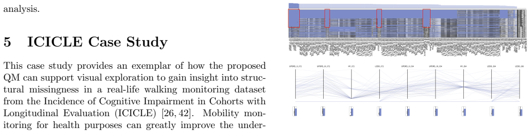
The paper's central claim is that structural missingness in large, high-dimensional data can be surfaced by six quality metrics defined over the three patterns of Amount Missing, Joint Missingness, and Conditional Missingness. $QAM$ gives each variable a score between 0 and 1 for the relative share of missing values. For each variable pair, $QJM_{mag}$ measures the observed share of jointly missing items, $QJM_{dir}$ measures the signed difference between observed and expected joint missingness, and $QJM_{abs}$ measures the absolute size of that deviation. For each directed pair, $QCM_{DiD}$ compares the distribution of recorded values for items that are missing in the other variable against the overall distribution, while $QCM_H$ compares their Shannon entropies. The paper demonstrates that mapping these values to variable ordering, subset selection, node size, edge width and colour, and histogram/glyph displays lets users spot clusters of attributes whose missingness is too structured to be random. In the ICICLE case study, the metrics expose blocks of missingness tied to study protocol, such as clinical measures not recorded for healthy controls and mutually exclusive activity-measurement sessions, and point to a testable hypothesis that declining health caused later dropouts.

Load-bearing premise

The load-bearing premise is that the two conditional-missingness metrics give dependable signals even when only a handful of items are missing in one variable but recorded in the other; the paper itself notes in Section 5.4 that with high joint missingness these scores are forced high and uses an ad-hoc filter to suppress that effect.

Editorial extensions

If this is right

Ordering variables by $QAM$ immediately separates attributes whose missingness would make simple imputation unreliable from those that are nearly complete.
Pairs with high $QJM_{abs}$ and clearly positive or negative $QJM_{dir}$ can be prioritized for data-collection debugging, since their co-missingness cannot be explained by per-variable missing rates alone.
High $QCM$ values in a direction $\vec d_j \to \vec d_k$ give an evidence-based reason to impute $\vec d_j$ using recorded values in $\vec d_k$, or to withhold imputation and model the missingness explicitly.
The same metrics can be applied to categorical variables by treating categories as histogram bins, extending the method beyond numerical sensor data.
In longitudinal studies, trends in $QAM$ and $QJM_{abs}$ across time points can track worsening cohort health or protocol drift as the study ages.

Reading between the lines

Editorial extensions of the paper, not claims the author makes directly.

The deviation-from-chance framing of $QJM_{dir}$ could be reused for any pairwise co-absence problem, such as co-occurring sensor failures or mutually exclusive survey response patterns; the paper does not state this application.
The known instability of $QCM_{DiD}$ and $QCM_H$ when the conditioning subset is tiny suggests a natural extension: report a minimum-support count or confidence interval alongside each conditional score, and calibrate thresholds per dataset rather than using fixed cutoffs.
A null-model test that permutes missingness within each variable while preserving marginal missing rates could turn these metrics into formal significance tests of non-random missingness; that test is not in the paper.
If applied at the item level rather than the variable level, the metrics could flag individual records whose missingness profile is anomalous, a direction the paper does not explore.

Share X Bluesky LinkedIn Reddit HN

Editorial analysis

A structured set of objections, weighed in public.

Desk editor's note, referee report, and a circularity audit.

Desk Editor's Note

read the letter

Honest take: this is a useful formalization paper, not a breakthrough. The six quality metrics (equations 1–6) are clearly defined and correctly normalized, and they give missing-data visualization a simple ordering/ranking layer that was missing. The authors build on Fernstad's earlier taxonomy and add the actual equations, which is a legitimate contribution. The synthetic data and the ICICLE Parkinson's case study are both included, and the supplemental materials are available, which I appreciate.

The weak spots are both in the evaluation. First, the synthetic validation is circular in a real sense: they plant missingness patterns using the same quantities the metrics measure, so the metrics trivially recover them. That's a sanity check, not proof of usefulness. Second, and more consequential for the case study, the conditional-missingness metrics QCM_DiD and QCM_H compare a full distribution against a small subset S = DRk∩DMj. Section 5.4 acknowledges the small-sample problem, but the proposed fix—filtering on QJM_dir < 0.05 and QCM_DiD > 0.9—doesn't control |S|. Your stress test is right: with low QJM_dir, |S| ≈ P(dj missing)(1 − P(dk missing)), which can be tiny. The thresholds look chosen once, with no sensitivity analysis or null model. So the case-study claims about BMI, Height, and MoCA are weaker than the authors present. They are honest about the limitation, and they call the findings speculative, but the method doesn't yet have a way to distinguish real conditional structure from finite-sample noise.

The metrics themselves are not deep statistics—marginal proportion, independence deviations, total variation distance, entropy difference—but that's not a flaw; packaging them for visual guidance is the contribution. People working on missing-data visualization or data-quality triage in high-dimensional health data will get value from this. I'd like to see the authors add a sampling distribution or permutation-based null for QCM, and test the filter more systematically. I'd send this to peer review rather than desk reject: the formalization is clean, the visualization examples are instructive, and the real dataset is a plus. With a sensitivity analysis and a more careful treatment of the small-S case, it could be a solid reference for missing-data visualization work.

Referee Report

2 major / 5 minor

Summary. The paper defines six quality metrics for missingness patterns—QAM, QJM_mag, QJM_dir, QJM_abs, QCM_DiD, and QCM_H—and demonstrates their use in variable ordering, filtering, and network, parallel-coordinates, and MissiG visualizations. Section 3 gives the definitions, Section 4 presents synthetically generated datasets with controlled missingness structures, and Section 5 applies the metrics to the ICICLE walking-monitoring dataset, reporting structures that are traced to data-collection procedures. The paper also acknowledges in Section 5.4 that the conditional-missingness metrics are problematic when the conditioning subset is small. The central claim is that these metrics can guide visual exploration of structured missingness in large high-dimensional data.

Significance. The contribution is potentially valuable: quality metrics tailored to missingness structures are a genuine gap in the visualization literature, and the proposed metrics are clearly specified and correctly normalized, including the division by 2 in Eq. (5) and by log(bk) in Eq. (6). The visual encodings are sensible, and the ICICLE case study is a rich real-world exemplar. The supplemental materials with synthetic datasets are a useful asset. However, the validation is not yet strong enough to support the effectiveness claim: the synthetic experiments largely confirm quantities that were planted using the same definitions, and the conditional-missingness metrics lack uncertainty quantification or a null-model baseline.

major comments (2)

[§4.1, Tables 1–2; §4.3–§4.4] The synthetic evaluation plants missingness using exactly the quantities the metrics measure: JM patterns are generated by setting P(dj,dk) relative to E(dj,dk), which is what QJM_dir and QJM_abs compute by definition, and CM patterns are generated by placing missing values in predetermined value ranges, which is what QCM_DiD and QCM_H detect. The agreement reported in Sections 4.3 and 4.4 therefore confirms internal consistency, not detection power. Without a null model (e.g., MCAR replicates) or a comparison to standard missingness tests, the experiments do not establish that the metrics can distinguish structured missingness from chance, which is the central claim of Section 3. Please add a randomized-baseline evaluation reporting detection rates, precision/recall, or an equivalent performance measure.
[§5.4; Eqs. (5)–(6)] The CM metrics estimate a histogram and an entropy from the subset DRk∩DMj. When this subset is small, QCM_DiD is positively biased and QCM_H is inflated by the negative small-sample bias of sample entropy, so high values do not necessarily imply conditional missingness. Section 5.4 correctly acknowledges this for high joint missingness, but the proposed filter QJM_dir < 0.05 does not control the subset size: writing P(both) for P(DMj∩DMk), the conditioning subset has size P(DMj) − P(both), which under near-independence is approximately P(DMj)(1−P(DMk)) and can be tiny even when QJM_dir is near zero. The thresholds 0.05 and 0.9 are applied once, with no sensitivity analysis or null distribution, and the case-study conclusions about Height, BMI, and MoCA rest on the surviving edges. Please provide a sampling distribution or an explicit minimum-support criterion for Eqs. (5)–(6), and validate the filter on synthetic data with known small-S regimes.

minor comments (5)

[§4.1] The dataset is described as containing 106 patients, but 64 cancer patients plus 52 healthy controls sums to 116; please correct this inconsistency.
[Table 1] The last row reports '38.3.1%' where a valid percentage is intended; please fix this typographical error.
[§4.1] The phrase 'aN aNstrings' appears throughout; it should read 'NaN strings'.
[§5.4 and figure captions] There are several typographical slips, including 'furhtermore' and 'zoomed in in figure 14'; these should be cleaned up before publication.
[§5.4] The text describes the filter QJM_dir < 0.05 as indicating low joint missingness, but QJM_dir is a signed deviation from expected joint missingness, not a magnitude; the wording should clarify that the filter is selecting a mix of negative and small positive deviations.

Circularity Check

0 steps flagged · score 0.0 of 10

No significant circularity: the paper defines explicit quality metrics and demonstrates them on synthetic and real data; no prediction or fitted parameter reduces to its own inputs.

full rationale

The paper's contribution is a set of explicit quality-metric definitions (Eqs. 1-6), not a derivation of a population quantity from a fitted model. QAM is the missingness proportion, QJM_mag the joint missingness proportion, QJM_dir/QJM_abs the signed and absolute deviations from the independence baseline E(dj,dk)=P(dj)P(dk), and QCM_DiD/QCM_H are total-variation and normalized-entropy differences between a marginal and a conditional histogram. These are transparent, closed-form functions of the data; no parameter is fitted to a subset and then renamed as a prediction. The synthetic experiments in Section 4.1 plant missingness patterns using the very quantities the metrics report, e.g. setting P(dj,dk) equal to, above, or below E(dj,dk) for QJM_dir, but this is a controlled sanity check with known ground truth, not a circular derivation: the paper does not claim to predict the planted patterns from the metrics; it displays the metrics on data whose structure is already known. The ICICLE case study provides an external, real-world demonstration, and Section 5.4 openly acknowledges that QCM_DiD and QCM_H become unstable when the conditioning subset DRk ∩ DMj is small, proposing an explicit filter rather than claiming the raw metrics are universally valid. That limitation is a robustness or statistical-inference concern, not circularity. Self-citations to [16] and [11] supply background definitions of missingness patterns and the MissiG glyph design, but the validity of Eqs. 1-6 does not rest on those citations: the equations are stated in full and are computable from the data alone. No uniqueness theorem, ansatz smuggled in via citation, or renaming of a known result is used to force the paper's conclusions. The case-study findings are explicitly speculative and exploratory, further reducing any sense of a derived prediction. Overall, the derivation chain, to the extent there is one, is self-contained and non-circular.

Assumptions & free parameters 3 free parameters · 3 assumptions · 0 invented entities

The metrics themselves have no internal free parameters, but the case-study workflow adds analyst-chosen thresholds, and the synthetic validation relies on generation parameters. The main axioms are the sufficiency of the AM, JM, and CM taxonomy, the product-of-marginals independence baseline, and the assumption that sparse conditional subsets still support distribution comparison; the paper itself shows the last one can fail in Section 5.4.

free parameters (3)

Edge filter thresholds for CM exploration = QJM_dir < 0.05 and QCM_DiD > 0.9
Chosen by the authors in Section 5.4 to isolate candidate conditional-missingness pairs in ICICLE; no sensitivity analysis or principled selection criterion is given. The network in Figure 12 and the conditional-missingness findings depend on these thresholds.
Attribute selection thresholds in case study = top 9 and top 23 attributes by QAM or QJM_abs
In Sections 5.2 and 5.3, barchart thresholding selects subsets for parallel-coordinate and glyph views; the exact cutoffs are set interactively and are not justified.
Synthetic missingness generation parameters = missingness 0 to 50 percent for AM, 20 to 50 percent for JM, 10 to 33 percent for CM; CM strengths 30, 60, and 90…
Section 4.1 uses these hand-chosen parameters to create the controlled datasets. They are not varied systematically, so the evaluation does not test how metric values respond across a range of realistic missingness regimes.

assumptions (3)

domain assumption The three pattern classes Amount Missing, Joint Missingness, and Conditional Missingness are the relevant structure taxonomy for missingness analysis.
The paper builds directly on Johansson Fernstad [16], which defines these patterns. The metrics are only as complete as the taxonomy, and no evidence is given that other missingness structures, such as hierarchical or time-series-specific patterns, are covered.
domain assumption Expected joint missingness under chance is the product of the two variables' marginal missingness probabilities, E(dj,dk) = P(dj)P(dk).
Used in equations 2 through 4 to define QJM_dir and QJM_abs. The interpretation of deviations as non-random structure assumes independence of missingness indicators, and the metric does not test significance or account for sample size.
domain assumption Comparing the distribution of dk for items missing in dj with the overall distribution of dk reveals conditional missingness.
Equations 5 and 6 define this comparison. The paper itself reports in Section 5.4 that the comparison becomes unreliable when the subset DRk ∩ DMj is sparse due to high joint missingness.

how reviews work

0 comments

Cite this review

Pith. "Pith review of To Measure What Isn't There -- Visual Exploration of Missingness Structures Using Quality Metrics." pith.science (2026). https://pith.science/paper/OAVZE5U5

@misc{pith2026250523447,
  author       = {Pith},
  title        = {Pith review of: To Measure What Isn't There -- Visual Exploration of Missingness Structures Using Quality Metrics},
  year         = {2026},
  howpublished = {\url{https://pith.science/paper/OAVZE5U5}},
  note         = {Machine review of arXiv:2505.23447}
}

read the original abstract

This paper contributes a set of quality metrics for identification and visual analysis of structured missingness in high-dimensional data. Missing values in data are a frequent challenge in most data generating domains and may cause a range of analysis issues. Structural missingness in data may indicate issues in data collection and pre-processing, but may also highlight important data characteristics. While research into statistical methods for dealing with missing data are mainly focusing on replacing missing values with plausible estimated values, visualization has great potential to support a more in-depth understanding of missingness structures in data. Nonetheless, while the interest in missing data visualization has increased in the last decade, it is still a relatively overlooked research topic with a comparably small number of publications, few of which address scalability issues. Efficient visual analysis approaches are needed to enable exploration of missingness structures in large and high-dimensional data, and to support informed decision-making in context of potential data quality issues. This paper suggests a set of quality metrics for identification of patterns of interest for understanding of structural missingness in data. These quality metrics can be used as guidance in visual analysis, as demonstrated through a use case exploring structural missingness in data from a real-life walking monitoring study. All supplemental materials for this paper are available at https://doi.org/10.25405/data.ncl.c.7741829.

Figures

Figures reproduced from arXiv: 2505.23447 by the authors.

**Figure 2.** The basic structure of MissiG for three or four vari [PITH_FULL_IMAGE:figures/full_fig_p005_2.png] view at source ↗

**Figure 3.** Visualization of BreastCancerAM. Missing values are represented below the axes in PC, and MissiG glyphs are used to display further missingness structures [PITH_FULL_IMAGE:figures/full_fig_p007_3.png] view at source ↗

Figures from the paper (8 more)

**Figure 4.** Figure 4: BreastCancerJM displayed in heatmap and barchart ordered from left to right by QAM. work use a spring embedded layout with QJMabs as edge weight. Deviations from expected JM are further emphasized through edge width based on QJMabs, and edge colouring by QJMdir with…

**Figure 7.** Figure 7: Network visualization of [PITH_FULL_IMAGE:figures/full_fig_p008_7.png]

**Figure 8.** Figure 8: Visualization of BreastCancerCM ordered by QCMh. MCP 1 is selected in all views, and items with missing values in MCP 1 are highlighted in red in PC and MissiG. out is used with ordering based on QAM and edge width and colour based on QCMh values of the variable pairs…

**Figure 9.** Figure 9: The 206 attributes of the ICICLE dataset ordered [PITH_FULL_IMAGE:figures/full_fig_p009_9.png]

**Figure 10.** Figure 10: Visual analysis of Joint Missingness structures in the ICICLE dataset. The 206 attributes are ordered by the [PITH_FULL_IMAGE:figures/full_fig_p010_10.png]

**Figure 11.** Figure 11: Network visualization of the ICICLE dataset with [PITH_FULL_IMAGE:figures/full_fig_p010_11.png]

**Figure 13.** Figure 13: Visualization of the subset of variable pairs with [PITH_FULL_IMAGE:figures/full_fig_p011_13.png]

**Figure 14.** Figure 14: The MissiG representation for MoCA total t72 (14a), MoCA total t18 (14b) and MoCA total t0 (14c) with missing in Ax Lb I Si Stance mu t36 highlighted (zoomed in from figure 13. ing values in Ax Lb I Si Stance mu t36, as represented by the red histograms in the MissiG …

Discussion (0). Sign in to comment.

Reference graph

Works this paper leans on

43 extracted references · 42 canonical work pages

[1]

Alsufyani, M

S. Alsufyani, M. Forshaw, S. Del Din, A. Yarnall, L. Rochester, and S. J. Fernstad. Multi-level visualiza- tion for exploration of structures in missing data. Com- puter Graphics and Visual Computing (CGVC). The Eu- rographics Association, 2024

work page 2024
[2]

Alsufyani, M

S. Alsufyani, M. Forshaw, and S. Johansson Fernstad. Visualization of missing data: a state-of-the-art survey. arXiv preprint arXiv:2410.03712 , 2024

arXiv 2024
[3]

Andreasson and M

R. Andreasson and M. Riveiro. Effects of visualizing missing data: an empirical evaluation. In 2014 18th International Conference on Information Visualisation , pp. 132–138. IEEE, 2014

work page 2014
[4]

A. O. Artero, M. C. F. de Oliveira, and H. Levkowitz. Enhanced high dimensional data visualization through dimension reduction and attribute arrangement. In Tenth International Conference on Information Visuali- sation (IV’06) , pp. 707–712. IEEE, 2006

work page 2006
[5]

B¨ auerle, C

A. B¨ auerle, C. van Onzenoodt, S. der Kinderen, J. J. Westberg, D. J¨ onsson, and T. Ropinski. Where did my lines go? visualizing missing data in parallel coordinates. In Computer Graphics Forum, vol. 41, pp. 235–246. Wi- ley Online Library, 2022

work page 2022
[6]

R. A. Becker and W. S. Cleveland. Brushing scatterplots. Technometrics, 29(2):127–142, May 1987

work page 1987
[7]

Behrisch, M

M. Behrisch, M. Blumenschein, N. W. Kim, L. Shao, M. El-Assady, J. Fuchs, D. Seebacher, A. Diehl, U. Bran- des, H. Pfister, et al. Quality metrics for information visualization. In Computer Graphics Forum, vol. 37, pp. 625–662. Wiley Online Library, 2018

work page 2018
[8]

Bertini, A

E. Bertini, A. Tatu, and D. Keim. Quality metrics in high-dimensional data visualization: An overview and systematization. Visualization and Computer Graphics, IEEE Transactions on, 17(12):2203–2212, 2011

work page 2011

Show all 43 references

[9]

Carpenter and M

J. Carpenter and M. Kenward. Multiple Imputation and its Application. Wiley, 2013

2013
[10]

Djurcilov and A

S. Djurcilov and A. Pang. Visualizing sparse gridded data sets. IEEE Computer Graphics and Applications , 20(5):52–57, 2000

2000
[11]

S. J. Fernstad and J. J. Westberg. To explore what isn’t there — glyph-based visualization for analysis of missing values. IEEE Transactions on Visualization and Com- puter Graphics, 28(10):3513–3529, 2021

2021
[12]

Fielding, P

S. Fielding, P. M. Fayers, and C. R. Ramsay. Investi- gating the missing data mechanism in quality of life out- comes: a comparison of approaches. Health and Quality of Life Outcomes , 7(1):57, 2009

2009
[13]

Inselberg

A. Inselberg. The plane with parallel coordinates. The Visual Computer , 1(4):69–91, 1985

1985
[14]

Jim´ enez and R

E. Jim´ enez and R. Mac ´ ıas. Graphical tools for visualiza- tion of missing data in large longitudinal phenomena. In Computer Graphics Forum , vol. 41, pp. 438–452. Wiley Online Library, 2022

2022
[15]

Johansson and J

S. Johansson and J. Johansson. Interactive dimensional- ity reduction through user-defined combinations of qual- ity metrics. IEEE Transactions on Visualization and Computer Graphics, 15(6):993–1000, 2009. 12

2009
[16]

Johansson Fernstad

S. Johansson Fernstad. To identify what isn’t there: A definition of missingness patterns and evaluation of missing value visualization. Information Visualization , 18(2):230–250, 2019

2019
[17]

Johansson Fernstad and R

S. Johansson Fernstad and R. C. Glen. Visual analy- sis of missing data – to see what isn’t there. In Poster Proceedings of IEEE Vis. IEEE, November 2014

2014
[18]

Johansson Fernstad, J

S. Johansson Fernstad, J. Johansson, S. Adams, J. Shaw, and D. Taylor. Visual exploration of microbial popula- tions. In Proceedings of IEEE Symposium on Biological Data Visualization , pp. 127–134. IEEE, October 2011

2011
[19]

Johansson Fernstad, A

S. Johansson Fernstad, A. Macquisten, J. Berrington, N. Embleton, and C. Stewart. Quality metrics to guide visual analysis of high dimensional genomics data. In EuroVis Workshop On Visual Analytics (EuroV A), 2020

2020
[20]

Johansson Fernstad, J

S. Johansson Fernstad, J. Shaw, and J. Johansson. Quality-based guidance for exploratory dimensionality reduction. Information Visualization , 12(1):44–64, Jan 2013

2013
[21]

Krause, A

J. Krause, A. Dasgupta, J.-D. Fekete, and E. Bertini. Seekaview: An intelligent dimensionality reduction strat- egy for navigating high-dimensional data spaces. In LDA V 2016-IEEE 6th Symposium on Large Data Anal- ysis and Visualization , 2016

2016
[22]

Kullback and R

S. Kullback and R. A. Leibler. On information and suffi- ciency. The Annals of Mathematical Statistics , 22(1):79– 86, 1951

1951
[23]

D. J. Lehmann, S. Hundt, and H. Theisel. A study on quality metrics vs. human perception: Can visual measures help us to filter visualizations of interest? it- Information Technology, 57(1):11–21, 2015

2015
[24]

J. M. Lewis, M. Ackerman, and V. R. de Sa. Human cluster evaluation and formal quality measures: A com- parative study. In CogSci, pp. 1870–1875, 2012

2012
[25]

S. Liu, D. Maljovec, B. Wang, P.-T. Bremer, and V. Pas- cucci. Visualizing high-dimensional data: Advances in the past decade. IEEE Transactions on Visualization and Computer Graphics , 23(3):1249–1268, 2017

2017
[26]

S. Lord, B. Galna, S. Coleman, A. Yarnall, D. Burn, and L. Rochester. Cognition and Gait Show a Selective Pat- tern of Association Dominated by Phenotype in Incident Parkinson’s Disease. Frontiers in Aging Neuroscience, 6, Oct. 2014. doi: 10.3389/fnagi.2014.00249

2014
[27]

Patr ´ ıcio, J

M. Patr ´ ıcio, J. Pereira, J. Cris´ ostomo, P. Matafome, M. Gomes, R. Sei¸ ca, and F. Caramelo. Using resistin, glucose, age and bmi to predict the presence of breast cancer. BMC cancer, 18(1):29, 2018

2018
[28]

D. B. Rubin. Inference and missing data. Biometrika, 63(3):581–592, 1976

1976
[29]

Sedlmair, A

M. Sedlmair, A. Tatu, T. Munzner, and M. Tory. A tax- onomy of visual cluster separation factors. In Computer Graphics Forum, vol. 31, pp. 1335–1344. Wiley Online Library, 2012

2012
[30]

C. E. Shannon. A mathematical theory of communica- tion. The Bell System Technical Journal , 17(3):379–423, 1948

1948
[31]

Shannon, A

P. Shannon, A. Markiel, O. Ozier, N. S. Baliga, J. T. Wang, D. Ramage, N. Amin, B. Schwikowski, and T. Ideker. Cytoscape: a software environment for in- tegrated models of biomolecular interaction networks. Genome research, 13(11):2498–2504, 2003

2003
[32]

Shimazaki and S

H. Shimazaki and S. Shinomoto. A method for selecting the bin size of a time histogram. Neural Computation , 19(6):1503–1527, 2007

2007
[33]

H. Song, Y. Fu, B. Saket, and J. Stasko. Understanding the effects of visualizing missing values on visual data ex- ploration. In 2021 IEEE Visualization Conference (VIS), pp. 161–165. IEEE, 2021

2021
[34]

Song and D

H. Song and D. A. Szafir. Where’s my data? evaluat- ing visualizations with missing data. IEEE transactions on visualization and computer graphics , 25(1):914–924, 2018

2018
[35]

Tierney and D

N. Tierney and D. Cook. Expanding tidy data principles to facilitate missing data exploration, visualization and assessment of imputations. Journal of Statistical Soft- ware, 105:1–31, 2023

2023
[36]

Turkay, P

C. Turkay, P. Filzmoser, and H. Hauser. Brushing dimen- sions – a dual visual analysis model for high-dimensional data. IEEE Transactions on Visualization and Computer Graphics, 17(12):2591–2599, 2011

2011
[37]

Turkay, J

C. Turkay, J. Parulek, and H. Hauser. Dual analysis of dna microarrays. In Proceedings of the 12th International Conference on Knowledge Management and Knowledge Technologies, pp. 26:1–26:8, 2012

2012
[38]

Valero-Mora, M

P. Valero-Mora, M. F. Rodrigo, M. Sanchez, and J. San- Martin. A plot for the visualization of missing value patterns in multivariate data. Practical Assessment, Re- search, and Evaluation , 24(1):9, 2019

2019
[39]

Wang and S

H. Wang and S. Wang. Visualization of the critical pat- terns of missing values in classification data. In Advances in Visual Information Systems , pp. 267–274. Springer, 2007

2007
[40]

Wang and S

H. Wang and S. Wang. Data mining with incomplete data. In Encyclopedia of Data Warehousing and Mining , pp. 526–530. IGI Global, second ed., 2009

2009
[41]

J. Wang, X. Liu, and H. W. Shen. High-dimensional data analysis with subspace comparison using matrix visual- ization. Information Visualization , 18(1):94–109, 2019. doi: 10.1177/1473871617733996

2019 doi
[42]

A. J. Yarnall, D. P. Breen, G. W. Duncan, S. Y. Cole- man, C. Nombela, T. W. Robbins, K. Wesnes, D. J. Brooks, R. A. Barker, and D. J. Burn. Characterizing mild cognitive impairment in incident Parkinson disease: The ICICLE-PD Study. Neurology, 82(4):308–316, Jan
[2014]

doi: 10.1212/WNL.0000000000000066 13

doi

Pith tools

Reviewed August 7, 2026 · model on record in the stance chip above.

[1] [1]

Alsufyani, M

S. Alsufyani, M. Forshaw, S. Del Din, A. Yarnall, L. Rochester, and S. J. Fernstad. Multi-level visualiza- tion for exploration of structures in missing data. Com- puter Graphics and Visual Computing (CGVC). The Eu- rographics Association, 2024

work page 2024

[2] [2]

Alsufyani, M

S. Alsufyani, M. Forshaw, and S. Johansson Fernstad. Visualization of missing data: a state-of-the-art survey. arXiv preprint arXiv:2410.03712 , 2024

arXiv 2024

[3] [3]

Andreasson and M

R. Andreasson and M. Riveiro. Effects of visualizing missing data: an empirical evaluation. In 2014 18th International Conference on Information Visualisation , pp. 132–138. IEEE, 2014

work page 2014

[4] [4]

A. O. Artero, M. C. F. de Oliveira, and H. Levkowitz. Enhanced high dimensional data visualization through dimension reduction and attribute arrangement. In Tenth International Conference on Information Visuali- sation (IV’06) , pp. 707–712. IEEE, 2006

work page 2006

[5] [5]

B¨ auerle, C

A. B¨ auerle, C. van Onzenoodt, S. der Kinderen, J. J. Westberg, D. J¨ onsson, and T. Ropinski. Where did my lines go? visualizing missing data in parallel coordinates. In Computer Graphics Forum, vol. 41, pp. 235–246. Wi- ley Online Library, 2022

work page 2022

[6] [6]

R. A. Becker and W. S. Cleveland. Brushing scatterplots. Technometrics, 29(2):127–142, May 1987

work page 1987

[7] [7]

Behrisch, M

M. Behrisch, M. Blumenschein, N. W. Kim, L. Shao, M. El-Assady, J. Fuchs, D. Seebacher, A. Diehl, U. Bran- des, H. Pfister, et al. Quality metrics for information visualization. In Computer Graphics Forum, vol. 37, pp. 625–662. Wiley Online Library, 2018

work page 2018

[8] [8]

Bertini, A

E. Bertini, A. Tatu, and D. Keim. Quality metrics in high-dimensional data visualization: An overview and systematization. Visualization and Computer Graphics, IEEE Transactions on, 17(12):2203–2212, 2011

work page 2011